DAQA - Extended analysis#
This analysis will answer the following questions…
For the whole data set:
what % of projects have addresses?
what % of projects have completion dates?
what % of projects have associated firms but no architects?
what % of projects have associated architects but no firms?
what % of firms have ‘operating years’ recorded
Number of projects:
Before 1940
Between 1940-1980
Post 1980
Undated
For the 40-80 data set:
what % of projects have addresses?
what % of projects have completion dates?
what % of projects have associated firms but no architects?
what % of projects have associated architects but no firms?
what % of firms have ‘operating years’ recorded
Analytic questions:
Which architects were associated with Queensland governement projects i.e., Brisbane City Council, Department of Works, etc.?
Which architects have registrations recorded in DAQA between 1940-1980?
UQ vs (BCTC, QIT, QUT) vs the rest for whole data, 1940-1980, and also 1940 to present.
Repeat ‘how many completed related to a person’. 1940-1980 and the Pareto distribution
Number completed projects 1940-80
Number of works by year, most active vs rest 1940-1980
what % of the different typologies 1940-1980
Number of works by year by typology
what % of projects extant/demolished/modified 1940-1980
average and mean number of employers of the DAQA interviewed architects
names of Architects associated with the highest number of projects 1940-1980
names of firms associated with the highest number of projects 1940-1980
names of top 5 Architects associated with the highest number of each typology 1940-1980
names of top 5 firms associated with the highest number of projects 1940-1980
what % of architects who are women associated with projects 1940-1980
what % of architects who are women associated with projects after 1980
5 Firms with the longest timespan with the same name.
5 Firms with the longest timespan with successive names/known predecessor firms.
Show code cell source
import requests, gzip, io, os, json

# for data mgmt
import pandas as pd
import numpy as np
from collections import Counter
from datetime import datetime
import ast

# for plotting
import matplotlib.pyplot as plt
from matplotlib.ticker import PercentFormatter
import plotly.graph_objects as go
import seaborn as sns
from matplotlib.colors import to_rgba
import plotly.express as px

# for hypothesis testing
from scipy.stats import chi2_contingency
from scipy.stats import pareto

import warnings
warnings.filterwarnings("ignore")

# provide folder_name which contains uncompressed data i.e., csv and jsonl files
# only need to change this if you have already downloaded data
# otherwise data will be fetched from google drive
global folder_name
folder_name = 'data/local'

def fetch_small_data_from_github(fname):
    url = f"https://raw.githubusercontent.com/acd-engine/jupyterbook/master/data/analysis/{fname}"
    response = requests.get(url)
    rawdata = response.content.decode('utf-8')
    return pd.read_csv(io.StringIO(rawdata))

def fetch_date_suffix():
    url = f"https://raw.githubusercontent.com/acd-engine/jupyterbook/master/data/analysis/date_suffix"
    response = requests.get(url)
    rawdata = response.content.decode('utf-8')
    try: return rawdata[:12]
    except: return None

def check_if_csv_exists_in_folder(filename):
    try: return pd.read_csv(os.path.join(folder_name, filename), low_memory=False)
    except: return None

def fetch_data(filetype='csv', acdedata='organization'):
    filename = f'acde_{acdedata}_{fetch_date_suffix()}.{filetype}'

    # first check if the data exists in current directory
    data_from_path = check_if_csv_exists_in_folder(filename)
    if data_from_path is not None: return data_from_path

    urls = fetch_small_data_from_github('acde_data_gdrive_urls.csv')
    sharelink = urls[urls.data == acdedata][filetype].values[0]
    url = f'https://drive.google.com/u/0/uc?id={sharelink}&export=download&confirm=yes'

    response = requests.get(url)
    decompressed_data = gzip.decompress(response.content)
    decompressed_buffer = io.StringIO(decompressed_data.decode('utf-8'))

    try:
        if filetype == 'csv': df = pd.read_csv(decompressed_buffer, low_memory=False)
        else: df = [json.loads(jl) for jl in pd.read_json(decompressed_buffer, lines=True, orient='records')[0]]
        return pd.DataFrame(df)
    except: return None

def fetch_all_DAQA_data():
    daqa_data_dict = dict()
    for entity in ['event', 'organization', 'person', 'place', 'recognition', 'resource', 'work']:
        daqa_this_entity = fetch_data(acdedata=entity)
        daqa_data_dict[entity] = daqa_this_entity[daqa_this_entity.data_source.str.contains('DAQA')]
    return daqa_data_dict

df_daqa_dict = fetch_all_DAQA_data() # 1 min if data is already downloaded
daqa_work = df_daqa_dict['work']
daqa_persons = df_daqa_dict['person']
daqa_orgs = df_daqa_dict['organization']
daqa_resources = df_daqa_dict['resource']
High-level summary of DAQA entities#
Before we jump into the analysis in response to the questions above, let’s take a look at a high-level of each DAQA entity i.e., person, organisation, work, resource.
Each entity has a class and we provide the count for each class for a given entity along with the total count of all classes. Next we output a count of all relationships between entities, and to this end, we generate detailled counts for all class-level relationships for each entity.
Show code cell source
# architects
print('Total number of persons:', daqa_persons.shape[0])
architect_count = daqa_persons['longterm_roles'].value_counts().reset_index()
architect_count['Proportion'] = round(architect_count['longterm_roles']/architect_count['longterm_roles'].sum(),3)
architect_count['Type'] = np.where(architect_count['index'].str.contains('non-architect'), 'non-architect', 'architect')
display(architect_count\
        .groupby('Type')\
        .sum()\
        .reset_index()\
        .rename(columns={'longterm_roles':'Frequency'})\
        .set_index('Type')
        .sort_values('Frequency', ascending=False))

# firms
print('\nTotal number of organisations:', daqa_orgs.shape[0])
firm_count = daqa_orgs['_class_ori'].value_counts().reset_index()
firm_count['Proportion'] = round(firm_count['_class_ori']/firm_count['_class_ori'].sum(),3)
display(firm_count\
        .groupby('index')\
        .sum()\
        .reset_index()\
        .rename(columns={'index':'Type', '_class_ori':'Frequency'})\
        .set_index('Type')
        .sort_values('Frequency', ascending=False))

# projects
print('\nTotal number of works i.e, projects:', daqa_work.shape[0])
project_count = daqa_work['_class_ori'].value_counts().reset_index()
project_count['Proportion'] = round(project_count['_class_ori']/project_count['_class_ori'].sum(),3)
display(project_count\
        .groupby('index')\
        .sum()\
        .reset_index()\
        .rename(columns={'index':'Type', '_class_ori':'Frequency'})\
        .set_index('Type')
        .sort_values('Frequency', ascending=False))

# articles
print('\nTotal number of resources i.e., articles, interviews:', daqa_resources.shape[0])
article_count = daqa_resources['_class_ori'].value_counts().reset_index()
article_count['Proportion'] = round(article_count['_class_ori']/article_count['_class_ori'].sum(),3)
display(article_count\
        .groupby('index')\
        .sum()\
        .reset_index()\
        .rename(columns={'index':'Type', '_class_ori':'Frequency'})\
        .set_index('Type')
        .sort_values('Frequency', ascending=False))
Total number of persons: 1103
| Frequency | Proportion | |
|---|---|---|
| Type | ||
| architect | 912 | 0.827 |
| non-architect | 191 | 0.173 |
Total number of organisations: 967
| Frequency | Proportion | |
|---|---|---|
| Type | ||
| "firm" | 907 | 0.938 |
| "education" | 39 | 0.040 |
| "organisation" | 15 | 0.016 |
| "government" | 6 | 0.006 |
Total number of works i.e, projects: 2203
| Frequency | Proportion | |
|---|---|---|
| Type | ||
| "structure" | 2203 | 1.0 |
Total number of resources i.e., articles, interviews: 7696
| Frequency | Proportion | |
|---|---|---|
| Type | ||
| "Photograph" | 3784 | 0.492 |
| "LineDrawing" | 1102 | 0.143 |
| "article" | 783 | 0.102 |
| "Image" | 742 | 0.096 |
| "Article" | 686 | 0.089 |
| "Audio" | 142 | 0.018 |
| "Transcript" | 128 | 0.017 |
| "Portrait" | 102 | 0.013 |
| "interview" | 92 | 0.012 |
| "Youtube" | 46 | 0.006 |
| "publication" | 46 | 0.006 |
| "Video" | 40 | 0.005 |
| "Spreadsheet" | 3 | 0.000 |
Show code cell source
relationship_cols = daqa_persons.iloc[:, 62:].columns
relevant_datasets = df_daqa_dict.keys()

relations = []
for this_df in relevant_datasets:
    for idx,row in df_daqa_dict[this_df].iterrows():
        for col in relationship_cols:
            try:
                if isinstance(row[col], str): relations.append(pd.json_normalize(ast.literal_eval(row[col])))
            except: continue

relations = pd.concat(relations)
relations = relations.drop_duplicates()

# replace person with specfic role
# create dictionary of architects and their ids
arch_nonarch_dict = daqa_persons[['ori_id','longterm_roles']]
arch_nonarch_dict['_class_ori'] = np.where(arch_nonarch_dict['longterm_roles'].str.contains('non-architect'), 'non-architect', 'architect')
arch_nonarch_dict = arch_nonarch_dict.drop('longterm_roles', axis=1).set_index('ori_id').to_dict()['_class_ori']

relations['subject.ori_id'] = relations['subject.ori_id'].astype(str)
relations['object.ori_id'] = relations['object.ori_id'].astype(str)

relations['subject._class_ori'] = np.where(relations['subject._class'] == 'person',
                                       relations['subject.ori_id'].map(arch_nonarch_dict),
                                       relations['subject._class_ori'])
relations['object._class_ori'] = np.where(relations['object._class'] == 'person',
                                       relations['object.ori_id'].map(arch_nonarch_dict),
                                       relations['object._class_ori'])

# relations
print('Total number of relationships:', relations.shape[0])
display(relations.relation_class.value_counts()\
        .reset_index()\
        .rename(columns={'index':'relation_class','relation_class':'Frequency'})\
        .assign(Proportion = lambda x: round(x['Frequency']/x['Frequency'].sum(),3))\
        .set_index('relation_class')
        .sort_values('Frequency', ascending=False))

# predicate terms
print('\nTotal number of unique predicates', relations['predicate.term'].nunique())
display(relations['predicate.term'].value_counts()\
        .reset_index()\
        .rename(columns={'index':'predicate.term','predicate.term':'Frequency'})\
        .assign(Proportion = lambda x: round(x['Frequency']/x['Frequency'].sum(),3))\
        .set_index('predicate.term')
        .sort_values('Frequency', ascending=False))
Total number of relationships: 17451
| Frequency | Proportion | |
|---|---|---|
| relation_class | ||
| Work_RelatedResource | 4889 | 0.280 |
| Person_RelatedWork | 2313 | 0.133 |
| Person_RelatedPerson | 1952 | 0.112 |
| Work_RelatedPlace | 1843 | 0.106 |
| Person_RelatedOrganization | 1568 | 0.090 |
| Organization_RelatedWork | 1484 | 0.085 |
| Resource_RelatedResource | 924 | 0.053 |
| Person_RelatedResource | 671 | 0.038 |
| Resource_RelatedPerson | 610 | 0.035 |
| Organization_RelatedOrganization | 420 | 0.024 |
| Resource_RelatedOrganization | 195 | 0.011 |
| Work_RelatedOrganization | 177 | 0.010 |
| Resource_RelatedWork | 90 | 0.005 |
| Organization_RelatedResource | 83 | 0.005 |
| Resource_RelatedPlace | 77 | 0.004 |
| Person_RelatedRecognition | 60 | 0.003 |
| Resource_RelatedRecognition | 48 | 0.003 |
| Work_RelatedPerson | 31 | 0.002 |
| Organization_RelatedPerson | 7 | 0.000 |
| Person_RelatedPlace | 7 | 0.000 |
| Recognition_RelatedOrganization | 1 | 0.000 |
| Work_RelatedRecognition | 1 | 0.000 |
Total number of unique predicates 33
| Frequency | Proportion | |
|---|---|---|
| predicate.term | ||
| HasMedia | 6300 | 0.361 |
| WorkedOn | 3502 | 0.201 |
| LocatedIn | 1843 | 0.106 |
| Employment | 1289 | 0.074 |
| Reference | 1188 | 0.068 |
| RelatedTo | 636 | 0.036 |
| WorkedWith | 402 | 0.023 |
| TaughtBy | 357 | 0.020 |
| InfluencedBy | 244 | 0.014 |
| StudiedWith | 243 | 0.014 |
| PrecededBy | 221 | 0.013 |
| KnewSocially | 203 | 0.012 |
| succeededby | 189 | 0.011 |
| KnewProfessionally | 132 | 0.008 |
| StudiedAt | 118 | 0.007 |
| IsInvolvedIn | 97 | 0.006 |
| PartnerOf | 83 | 0.005 |
| DoneIn | 77 | 0.004 |
| DesignedBy | 63 | 0.004 |
| CollaboratedWith | 48 | 0.003 |
| KnewOf | 42 | 0.002 |
| TravelledTo | 28 | 0.002 |
| Awarded | 22 | 0.001 |
| ClientOf | 21 | 0.001 |
| MentoredBy | 18 | 0.001 |
| Founded | 16 | 0.001 |
| Became | 15 | 0.001 |
| WasInfluenceBy | 14 | 0.001 |
| Attended | 12 | 0.001 |
| TaughtAt | 9 | 0.001 |
| MergedWith | 7 | 0.000 |
| Read | 6 | 0.000 |
| Authored | 6 | 0.000 |
Show code cell source
def fetch_relation_details(relation_types, relations=relations):
    this_relation = relations[relations['relation_class'].isin(relation_types)].fillna('-')
    print(f'Total number of {relation_types[0].replace("Related","").replace("_","-")} relations:', this_relation.shape[0])
    display(this_relation[['subject._class_ori','object._class_ori','predicate.term']]\
        .value_counts()\
        .reset_index()\
        .rename(columns={0:'Frequency'})\
        .sort_values('Frequency', ascending=False))

print('###################### PERSON RELATIONSHIPS ######################')
print('\n')
fetch_relation_details(['Person_RelatedWork','Work_RelatedPerson'])
print('\n')
fetch_relation_details(['Person_RelatedPerson'])
print('\n')
fetch_relation_details(['Person_RelatedOrganization','Organization_RelatedPerson'])
print('\n')
fetch_relation_details(['Person_RelatedResource','Resource_RelatedPerson'])
print('\n')
fetch_relation_details(['Person_RelatedRecognition'])
print('\n')
fetch_relation_details(['Person_RelatedPlace'])
print('\n')

print('###################### WORK RELATIONSHIPS ######################')
print('\n')
fetch_relation_details(['Work_RelatedResource','Resource_RelatedWork'])
print('\n')
fetch_relation_details(['Work_RelatedPlace'])
print('\n')
fetch_relation_details(['Work_RelatedRecognition'])
print('\n')

print('###################### ORGANISATION RELATIONSHIPS ######################')
print('\n')
fetch_relation_details(['Organization_RelatedWork','Work_RelatedOrganization'])
print('\n')
fetch_relation_details(['Organization_RelatedOrganization'])
print('\n')
fetch_relation_details(['Recognition_RelatedOrganization'])

print('###################### RESOURCE RELATIONSHIPS ######################')
print('\n')
fetch_relation_details(['Resource_RelatedResource'])
print('\n')
fetch_relation_details(['Resource_RelatedOrganization','Organization_RelatedResource'])
print('\n')
fetch_relation_details(['Resource_RelatedPlace'])
print('\n')
fetch_relation_details(['Resource_RelatedRecognition'])
print('\n')
###################### PERSON RELATIONSHIPS ######################


Total number of Person-Work relations: 2344
| subject._class_ori | object._class_ori | predicate.term | Frequency | |
|---|---|---|---|---|
| 0 | architect | structure | WorkedOn | 2157 |
| 1 | architect | structure | Reference | 97 |
| 2 | structure | architect | DesignedBy | 30 |
| 3 | architect | structure | InfluencedBy | 20 |
| 4 | architect | structure | StudiedAt | 8 |
| 5 | architect | structure | Employment | 7 |
| 6 | architect | structure | TravelledTo | 6 |
| 7 | architect | structure | TaughtAt | 4 |
| 9 | architect | structure | Attended | 3 |
| 8 | architect | structure | RelatedTo | 3 |
| 10 | architect | structure | KnewOf | 2 |
| 11 | non-architect | structure | Reference | 2 |
| 12 | architect | structure | Read | 1 |
| 13 | architect | structure | ClientOf | 1 |
| 14 | architect | structure | WorkedWith | 1 |
| 15 | non-architect | structure | WorkedOn | 1 |
| 16 | structure | architect | ClientOf | 1 |
Total number of Person-Person relations: 1952
| subject._class_ori | object._class_ori | predicate.term | Frequency | |
|---|---|---|---|---|
| 0 | architect | architect | WorkedWith | 359 |
| 1 | architect | architect | TaughtBy | 323 |
| 2 | architect | architect | Reference | 219 |
| 3 | architect | architect | StudiedWith | 210 |
| 4 | architect | architect | InfluencedBy | 192 |
| 5 | architect | architect | KnewSocially | 171 |
| 6 | architect | architect | Employment | 97 |
| 7 | architect | architect | KnewProfessionally | 97 |
| 8 | architect | architect | KnewOf | 36 |
| 9 | architect | non-architect | KnewProfessionally | 32 |
| 10 | architect | non-architect | StudiedWith | 31 |
| 11 | architect | non-architect | KnewSocially | 29 |
| 12 | architect | non-architect | TaughtBy | 24 |
| 13 | architect | non-architect | CollaboratedWith | 16 |
| 14 | architect | architect | MentoredBy | 16 |
| 15 | architect | non-architect | WorkedWith | 15 |
| 17 | architect | non-architect | Reference | 14 |
| 16 | architect | architect | CollaboratedWith | 14 |
| 18 | architect | architect | WasInfluenceBy | 12 |
| 19 | non-architect | architect | ClientOf | 10 |
| 20 | architect | non-architect | InfluencedBy | 8 |
| 21 | architect | architect | PartnerOf | 8 |
| 22 | architect | architect | ClientOf | 4 |
| 23 | non-architect | non-architect | Employment | 2 |
| 24 | non-architect | non-architect | KnewProfessionally | 2 |
| 25 | architect | non-architect | Employment | 2 |
| 26 | architect | non-architect | MentoredBy | 2 |
| 27 | architect | architect | RelatedTo | 2 |
| 28 | non-architect | non-architect | KnewSocially | 2 |
| 29 | non-architect | architect | Employment | 1 |
| 30 | non-architect | architect | Reference | 1 |
| 31 | architect | non-architect | KnewOf | 1 |
Total number of Person-Organization relations: 1575
| subject._class_ori | object._class_ori | predicate.term | Frequency | |
|---|---|---|---|---|
| 0 | architect | firm | Employment | 1137 |
| 1 | architect | education | StudiedAt | 108 |
| 2 | architect | firm | PartnerOf | 75 |
| 3 | architect | firm | Reference | 55 |
| 4 | architect | education | Employment | 35 |
| 5 | architect | firm | InfluencedBy | 19 |
| 6 | architect | firm | Founded | 15 |
| 7 | architect | firm | WorkedWith | 14 |
| 8 | architect | firm | TaughtBy | 10 |
| 9 | architect | firm | CollaboratedWith | 9 |
| 10 | architect | education | Reference | 9 |
| 11 | architect | organisation | Became | 8 |
| 15 | architect | education | TaughtAt | 5 |
| 17 | architect | education | InfluencedBy | 5 |
| 16 | architect | education | CollaboratedWith | 5 |
| 13 | architect | government | WorkedWith | 5 |
| 14 | architect | education | Attended | 5 |
| 12 | architect | organisation | Reference | 5 |
| 18 | architect | organisation | RelatedTo | 4 |
| 19 | non-architect | firm | Employment | 4 |
| 20 | architect | organisation | WorkedWith | 3 |
| 21 | architect | education | Read | 3 |
| 27 | architect | education | Authored | 2 |
| 31 | architect | firm | StudiedWith | 2 |
| 30 | non-architect | firm | Reference | 2 |
| 29 | architect | education | TravelledTo | 2 |
| 28 | architect | firm | MergedWith | 2 |
| 24 | architect | education | WorkedWith | 2 |
| 26 | architect | organisation | Attended | 2 |
| 23 | firm | architect | ClientOf | 2 |
| 22 | architect | organisation | Employment | 2 |
| 25 | firm | architect | KnewOf | 2 |
| 40 | architect | education | ClientOf | 1 |
| 47 | architect | education | WorkedOn | 1 |
| 46 | architect | firm | KnewOf | 1 |
| 45 | architect | firm | KnewProfessionally | 1 |
| 44 | architect | firm | KnewSocially | 1 |
| 43 | architect | education | RelatedTo | 1 |
| 42 | architect | firm | WasInfluenceBy | 1 |
| 41 | architect | government | Employment | 1 |
| 38 | architect | education | Awarded | 1 |
| 39 | architect | organisation | CollaboratedWith | 1 |
| 37 | architect | firm | ClientOf | 1 |
| 36 | firm | architect | Became | 1 |
| 35 | non-architect | education | StudiedAt | 1 |
| 34 | non-architect | education | Employment | 1 |
| 33 | firm | architect | CollaboratedWith | 1 |
| 32 | firm | architect | MergedWith | 1 |
| 48 | non-architect | organisation | Founded | 1 |
Total number of Person-Resource relations: 1281
| subject._class_ori | object._class_ori | predicate.term | Frequency | |
|---|---|---|---|---|
| 0 | interview | architect | Reference | 364 |
| 1 | architect | Photograph | HasMedia | 257 |
| 2 | architect | interview | IsInvolvedIn | 91 |
| 3 | interview | architect | RelatedTo | 86 |
| 4 | non-architect | interview | RelatedTo | 86 |
| 5 | interview | non-architect | RelatedTo | 85 |
| 6 | architect | interview | RelatedTo | 82 |
| 7 | architect | Image | HasMedia | 80 |
| 8 | interview | non-architect | Reference | 75 |
| 9 | architect | Portrait | HasMedia | 66 |
| 10 | non-architect | interview | IsInvolvedIn | 6 |
| 11 | architect | LineDrawing | HasMedia | 1 |
| 12 | architect | publication | Reference | 1 |
| 13 | non-architect | Photograph | HasMedia | 1 |
Total number of Person-Recognition relations: 60
| subject._class_ori | object._class_ori | predicate.term | Frequency | |
|---|---|---|---|---|
| 0 | architect | award | Awarded | 20 |
| 1 | architect | award | TravelledTo | 15 |
| 2 | architect | award | Reference | 8 |
| 3 | architect | award | Became | 5 |
| 4 | architect | award | Authored | 3 |
| 5 | architect | award | Attended | 2 |
| 6 | architect | award | Read | 2 |
| 7 | architect | award | RelatedTo | 1 |
| 8 | architect | award | WasInfluenceBy | 1 |
| 9 | architect | award | WorkedWith | 1 |
| 10 | non-architect | award | Authored | 1 |
| 11 | non-architect | award | Reference | 1 |
Total number of Person-Place relations: 7
| subject._class_ori | object._class_ori | predicate.term | Frequency | |
|---|---|---|---|---|
| 0 | architect | place | TravelledTo | 5 |
| 1 | architect | place | Reference | 1 |
| 2 | architect | place | RelatedTo | 1 |
###################### WORK RELATIONSHIPS ######################


Total number of Work-Resource relations: 4979
| subject._class_ori | object._class_ori | predicate.term | Frequency | |
|---|---|---|---|---|
| 0 | structure | Photograph | HasMedia | 3143 |
| 1 | structure | LineDrawing | HasMedia | 1088 |
| 2 | structure | Image | HasMedia | 651 |
| 3 | interview | structure | Reference | 90 |
| 4 | structure | Portrait | HasMedia | 7 |
Total number of Work-Place relations: 1843
| subject._class_ori | object._class_ori | predicate.term | Frequency | |
|---|---|---|---|---|
| 0 | structure | place | LocatedIn | 1843 |
Total number of Work-Recognition relations: 1
| subject._class_ori | object._class_ori | predicate.term | Frequency | |
|---|---|---|---|---|
| 0 | structure | award | Awarded | 1 |
###################### ORGANISATION RELATIONSHIPS ######################


Total number of Organization-Work relations: 1661
| subject._class_ori | object._class_ori | predicate.term | Frequency | |
|---|---|---|---|---|
| 0 | firm | structure | WorkedOn | 1343 |
| 1 | structure | firm | RelatedTo | 144 |
| 2 | firm | structure | RelatedTo | 141 |
| 3 | structure | firm | DesignedBy | 33 |
Total number of Organization-Organization relations: 420
| subject._class_ori | object._class_ori | predicate.term | Frequency | |
|---|---|---|---|---|
| 0 | firm | firm | PrecededBy | 221 |
| 1 | firm | firm | succeededby | 189 |
| 2 | firm | firm | MergedWith | 4 |
| 3 | firm | firm | CollaboratedWith | 2 |
| 4 | firm | firm | WorkedWith | 2 |
| 5 | firm | firm | Became | 1 |
| 6 | government | firm | ClientOf | 1 |
Total number of Recognition-Organization relations: 1
| subject._class_ori | object._class_ori | predicate.term | Frequency | |
|---|---|---|---|---|
| 0 | award | education | StudiedAt | 1 |
###################### RESOURCE RELATIONSHIPS ######################


Total number of Resource-Resource relations: 924
| subject._class_ori | object._class_ori | predicate.term | Frequency | |
|---|---|---|---|---|
| 0 | article | Article | HasMedia | 646 |
| 1 | interview | Audio | HasMedia | 127 |
| 2 | interview | Transcript | HasMedia | 83 |
| 3 | interview | Youtube | HasMedia | 45 |
| 4 | interview | Video | HasMedia | 22 |
| 5 | interview | publication | Reference | 1 |
Total number of Resource-Organization relations: 278
| subject._class_ori | object._class_ori | predicate.term | Frequency | |
|---|---|---|---|---|
| 0 | interview | education | Reference | 121 |
| 1 | interview | firm | Reference | 68 |
| 2 | firm | Photograph | HasMedia | 57 |
| 3 | firm | Image | HasMedia | 15 |
| 4 | firm | Portrait | HasMedia | 9 |
| 5 | interview | organisation | Reference | 6 |
| 6 | firm | LineDrawing | HasMedia | 2 |
Total number of Resource-Place relations: 77
| subject._class_ori | object._class_ori | predicate.term | Frequency | |
|---|---|---|---|---|
| 0 | interview | place | DoneIn | 77 |
Total number of Resource-Recognition relations: 48
| subject._class_ori | object._class_ori | predicate.term | Frequency | |
|---|---|---|---|---|
| 0 | interview | award | Reference | 48 |
Projects & firms#
Below are some statistics about project characteristics and firms in the DAQA dataset. Proportions under the PROJECTS subheading are calculated as a percentage of the total number of projects in the dataset. Proportions under the FIRMS subheading are calculated as a percentage of the total number of firms in the dataset.
It should be noted that all people related to projects are architects, we found no non-architects in the project records. Also all organisations related to projects are firms, we found no non-firm organisations in the project records.
We define a project with an address as one that has a populated
addressfieldWe define a project with a geocode date as one that has a populated
longitudeandlatitudefieldWe define a project with a completion date as one that has a populated
completion yearfieldWe define a project with an associated firm as one that has a populated
related_organizationsfieldWe define a project with no associated firms as one that has a no populated
related organizationsfieldWe define a project with an associated architect as one that has a populated
related_peoplefieldWe define a project with no associated architects as one that has no populated
related_peoplefieldWe define a firm with operating years as an organisation that has a populated
operationfield
Show code cell source
print('###################### PROJECTS ######################')

# load data
daqa_work = df_daqa_dict['work']

print('\nQ: How many projects are recorded in DAQA?')
count_projects = len(daqa_work)
print(f'A: There are {count_projects} projects in DAQA.')

# we define a project with an address as one that has a populated "address" field
print('\nQ: what % of projects have addresses?')
count_projects_with_address = len(daqa_work[daqa_work.coverage_range.apply(lambda x: "address" in x)])
prop_projects_with_address = round((count_projects_with_address / count_projects) * 100, 2)
print(f'A: {prop_projects_with_address}% ({count_projects_with_address}) of DAQA projects have addresses.')

# we define a project with a geocode date as one that has a populated "longitude" field
print('\nQ: what % of projects have geocodes (lat/long)?')
count_projects_with_geocodes = len(daqa_work[daqa_work.coverage_range.apply(lambda x: "latitude" in x)])
prop_projects_with_geocodes = round((count_projects_with_geocodes / count_projects) * 100, 2)
print(f'A: {prop_projects_with_geocodes}% ({count_projects_with_geocodes}) of DAQA projects have geocodes.')

# we define a project with a completion date as one that has a populated "completion year" field
print('\nQ: what % of projects have completion dates?')
count_projects_with_completion_dates = len(daqa_work[daqa_work.coverage_range.apply(lambda x: "date_end" in x)])
prop_projects_with_completion_dates = round((count_projects_with_completion_dates / count_projects) * 100, 2)
print(f'A: {prop_projects_with_completion_dates}% ({count_projects_with_completion_dates}) of DAQA projects have completion dates.')

# we conduct a sanity check to see if related people in daqa_work are all architects, we find no non-architects
# # load data
# daqa_persons = df_daqa_dict['person']
# non_architects = daqa_persons[daqa_persons['longterm_roles'].str.contains('non-architect')]['ori_id'].unique()
# len(daqa_work[daqa_work.related_people.apply(lambda x: pd.json_normalize(eval(x))['subject.ori_id'].values[0] in non_architects if isinstance(x, str) else False)])

# we conduct a sanity check to see if related organisations in daqa_work are all firms, we find no non-firms
# count_related_organizations_firms = len(daqa_work[daqa_work.related_organizations.apply(lambda x: "firm" in x if isinstance(x, str) else False)])
# count_related_organizations = len(daqa_work[daqa_work.related_organizations.notnull()])
# count_related_organizations_firms == count_related_organizations

# we define a project with an associated firm as one that has a populated "related_organizations" field
print('\nQ: how many projects have associated firms?')
count_projects_with_firms = len(daqa_work[daqa_work.related_organizations.notnull()])
prop_projects_with_firms = round((count_projects_with_firms / count_projects) * 100, 2)
print(f'A: {prop_projects_with_firms}% ({count_projects_with_firms}) of DAQA projects have associated firms.')

# we define a project with no associated architects as one that has no populated "related_people" field
print('\nQ: what % of projects have associated firms but no architects?')
count_projects_with_firms_no_architects = len(daqa_work[(daqa_work.related_organizations.notnull()) &\
                                                        (daqa_work.related_people.isnull())])
prop_projects_with_firms_no_architects = round((count_projects_with_firms_no_architects / count_projects) * 100, 2)
print(f'A: {prop_projects_with_firms_no_architects}% ({count_projects_with_firms_no_architects}) of DAQA projects have associated firms but no architects.')

# we define a project with an associated architect as one that has a populated "related_people" field
print('\nQ: how many projects have associated architects?')
count_projects_with_architects = len(daqa_work[daqa_work.related_people.notnull()])
prop_projects_with_architects = round((count_projects_with_architects / count_projects) * 100, 2)
print(f'A: {prop_projects_with_architects}% ({count_projects_with_architects}) of DAQA projects have associated architects.')

# we define a project with an associated architects as one that has a populated "related people" field
# and we define a project with no associated firms as one that has a no populated "related organizations" field
print('\nQ: what % of projects have associated architects but no firms?')
count_projects_with_architects_no_firms = len(daqa_work[(daqa_work.related_organizations.isnull()) &\
                                                        (daqa_work.related_people.notnull())])
prop_projects_with_architects_no_firms = round((count_projects_with_architects_no_firms / count_projects) * 100, 2)
print(f'A: {prop_projects_with_architects_no_firms}% ({count_projects_with_architects_no_firms}) of DAQA projects have associated architects but no firms.')

print('\n###################### FIRMS ######################')

# load data
daqa_orgs = df_daqa_dict['organization']
daqa_firms = daqa_orgs[daqa_orgs['_class_ori'].str.contains('firm')].copy()

print('\nQ: How many firms are recorded in DAQA?')
count_firms = len(daqa_firms)
print(f'A: There are {count_firms} firms in DAQA.')

# we define an operating firm as an organisation that has a populated "operation" field with a start date
print('\nQ: what % of firms have ‘operating years’ recorded (just start)?')
count_firms_with_operating_start = len(daqa_firms[daqa_firms.operation.apply(lambda x: "date_start" in x if isinstance(x, str) else False)])
prop_firms_with_operating_start = round((count_firms_with_operating_start / count_firms) * 100, 2)
print(f'A: {prop_firms_with_operating_start}% ({count_firms_with_operating_start}) of DAQA firms have operating years recorded.')

# we define an operating firm as an organisation that has a populated "operation" field with start and end dates
print('\nQ: what % of firms have ‘operating years’ recorded (start and end)?')
count_firms_with_operating_years = len(daqa_firms[daqa_firms.operation.apply(lambda x: ("date_start" in x) & ("date_end" in x) if isinstance(x, str) else False)])
prop_firms_with_operating_years = round((count_firms_with_operating_years / count_firms) * 100, 2)
print(f'A: {prop_firms_with_operating_years}% ({count_firms_with_operating_years}) of DAQA firms have operating years recorded.')

# top 5 firms - longest timespan
daqa_firms_with_op_yrs = daqa_firms[daqa_firms.operation.apply(lambda x: "date_start" in x if isinstance(x, str) else False)]

# extract the start and end years from the "operation" field
start_dates = []; end_dates = []

for index, row in daqa_firms_with_op_yrs.iterrows():
    start_dates.append(int(pd.json_normalize(ast.literal_eval(row['operation']))['date_start.year'].values[0]))

    try: end_dates.append(int(pd.json_normalize(ast.literal_eval(row['operation']))['date_end.year'].values[0]))
    except: end_dates.append(None)

daqa_firms_with_op_yrs['start_yr'] = start_dates
daqa_firms_with_op_yrs['end_yr'] = end_dates
daqa_firms_with_op_yrs['diff'] = abs(daqa_firms_with_op_yrs['end_yr'] - daqa_firms_with_op_yrs['start_yr'])

print('\nQ: What are the top five firms with the longest timespan with the same name? (must have operating start and end years)')
display(daqa_firms_with_op_yrs.sort_values(by='diff', ascending=False)\
    .head(5)[['primary_name', 'start_yr', 'end_yr', 'diff']])
###################### PROJECTS ######################

Q: How many projects are recorded in DAQA?
A: There are 2203 projects in DAQA.

Q: what % of projects have addresses?
A: 84.29% (1857) of DAQA projects have addresses.

Q: what % of projects have geocodes (lat/long)?
A: 65.68% (1447) of DAQA projects have geocodes.

Q: what % of projects have completion dates?
A: 60.37% (1330) of DAQA projects have completion dates.

Q: how many projects have associated firms?
A: 58.87% (1297) of DAQA projects have associated firms.

Q: what % of projects have associated firms but no architects?
A: 14.21% (313) of DAQA projects have associated firms but no architects.

Q: how many projects have associated architects?
A: 81.03% (1785) of DAQA projects have associated architects.

Q: what % of projects have associated architects but no firms?
A: 36.36% (801) of DAQA projects have associated architects but no firms.

###################### FIRMS ######################

Q: How many firms are recorded in DAQA?
A: There are 907 firms in DAQA.

Q: what % of firms have ‘operating years’ recorded (just start)?
A: 79.93% (725) of DAQA firms have operating years recorded.

Q: what % of firms have ‘operating years’ recorded (start and end)?
A: 39.69% (360) of DAQA firms have operating years recorded.

Q: What are the top five firms with the longest timespan with the same name? (must have operating start and end years)
| primary_name | start_yr | end_yr | diff | |
|---|---|---|---|---|
| 21223 | "Evans Deakin & Company (Engineers & Shipbuild... | 1910 | 1980.0 | 70.0 |
| 21594 | "Bates Smart & McCutcheon" | 1926 | 1995.0 | 69.0 |
| 21165 | "Brown and Broad LTD" | 1905 | 1967.0 | 62.0 |
| 20909 | "Queensland Housing Commission" | 1945 | 2004.0 | 59.0 |
| 21164 | "George Brockwell Gill Architect and Agent" | 1889 | 1943.0 | 54.0 |
Top five firms with the longest timespan with successive names/known predecessor firms.#
We inspect the top five firms with the longest timespan with successive names/known predecessor firms. We use network graphs to visualise the predecessor/successor relationships between firms. The graphs are interactive, so you can click on the nodes to see the firm names and the years they were active.
Show code cell source
daqa_firms_with_related_orgs = daqa_firms[daqa_firms.related_organizations.notnull()]

related_orgs_df = pd.DataFrame()

for index, row in daqa_firms_with_related_orgs.iterrows():
    this_row_id = int(row['ori_id'])
    this_org_related = pd.json_normalize(ast.literal_eval(row['related_organizations']))
    related_orgs_df = related_orgs_df.append(this_org_related)

related_orgs_df.drop_duplicates(inplace=True)
related_orgs_df = related_orgs_df[related_orgs_df['predicate.term'].isin(['succeededby', 'PrecededBy','MergedWith'])]
related_orgs_ls = related_orgs_df[['subject.ori_id','object.ori_id']].values.tolist()

def get_connected_nodes(snapshot):
    connected_nodes = []
    for node_list in snapshot:
        connected_node_set = set(node_list)
        for connected_node in connected_nodes:
            if connected_node & connected_node_set:
                connected_node |= connected_node_set
                break
        else:
            connected_nodes.append(connected_node_set)

    connected_node_lists = [list(connected_node) for connected_node in connected_nodes]
    return connected_node_lists

connected_node_lists = get_connected_nodes(related_orgs_ls)
connected_node_lists = get_connected_nodes(connected_node_lists)
connected_node_lists = get_connected_nodes(connected_node_lists)

first_date = []
last_date = []

for nodes in connected_node_lists[0:]:
    this_nodes = daqa_firms_with_op_yrs[daqa_firms_with_op_yrs['ori_id'].astype(int).isin(nodes)]
    all_dates = this_nodes['start_yr'].to_list()
    all_dates.extend(this_nodes['start_yr'].to_list())

    if len(all_dates) > 0:
        first_date.append(min(all_dates))
        last_date.append(max(all_dates))

    else:
        first_date.append(None)
        last_date.append(None)


# dates
dts = pd.DataFrame([first_date, last_date]).T

# add nodes as column
dts.columns = ['first_date', 'last_date']
dts['nodes'] = connected_node_lists
dts['diff'] = dts['last_date'] - dts['first_date']

display(dts.sort_values(by='diff', ascending=False).head(5))
| first_date | last_date | nodes | diff | |
|---|---|---|---|---|
| 61 | 1862 | 1967 | [4795, 3838, 3846] | 105 |
| 4 | 1893 | 1995 | [2310, 2446, 2447, 2449, 4628, 2456, 2338, 502... | 102 |
| 2 | 1864 | 1963 | [5033, 2387, 2356, 2457, 4890, 4891, 4892, 4286] | 99 |
| 17 | 1926 | 2010 | [4576, 2497, 3868, 2440, 4459, 4460, 2445, 446... | 84 |
| 28 | 1938 | 2002 | [2336, 4994, 2501, 4511, 2413, 2478, 4527, 363... | 64 |
Firm 1 (105 years)
Show code cell source
def output_graph(data, iteration = 0):
    import networkx as nx
    from pyvis import network as net

    g = net.Network(notebook=True,
                    height='500px',
                    width="100%",
                    cdn_resources = 'remote',
                    select_menu=True)

    df = related_orgs_df[related_orgs_df['subject.ori_id']\
                    .isin(dts.sort_values(by='diff', ascending=False)\
                        .iloc[iteration]['nodes'])][['subject.label','object.label','predicate.term']]

    dd = daqa_firms_with_op_yrs.copy()
    dd['primary_name'] = dd['primary_name'].apply(lambda x: ast.literal_eval(x))

    # Iterate over each row in the dataset
    for _, row in df.iterrows():
        subject = row['subject.label']
        predicate = row['predicate.term']
        obj = row['object.label']

        try:
            sub_start = dd[dd['primary_name'].str.contains(subject)]['start_yr'].values[0]
            sub_end = dd[dd['primary_name'].str.contains(subject)]['end_yr'].values[0]
        except:
            sub_start = None
            sub_end = None

        try:
            obj_start = dd[dd['primary_name'].str.contains(obj)]['start_yr'].values[0]
            obj_end = dd[dd['primary_name'].str.contains(obj)]['end_yr'].values[0]
        except:
            obj_start = None
            obj_end = None

        g.add_node(subject, subject, title=f"{subject} \nStart: {sub_start} \nEnd: {sub_end}", color='blue')
        g.add_node(obj, obj, title=f"{obj} \nStart: {obj_start} \nEnd: {obj_end}", color='blue')

        # Add edges to the graph based on the relationship type
        if predicate == 'succeededby':
            g.add_edge(subject, obj, color='red', title=predicate, arrows='to')
        elif predicate == 'PrecededBy':
            g.add_edge(obj, subject, color='red', title='succeededby', arrows='to')
        elif predicate == 'MergedWith':
            g.add_edge(subject, obj, color='green', title=predicate, width=3)
            g.add_edge(obj, subject, color='green', title=predicate, width=3)

    var_options = """var_options = {
                    "nodes": {"font": {"size": 12}},
                    "interaction": {"hover": "True"}}
                """

    g.set_options(var_options)
    return g

display(daqa_firms_with_op_yrs[daqa_firms_with_op_yrs['ori_id'].astype(int)\
                       .isin(dts.sort_values(by='diff', ascending=False)\
                             .iloc[0]['nodes'])][['primary_name','ori_id','start_yr','end_yr']]\
                        .sort_values(by='start_yr', ascending=True))

g = output_graph(related_orgs_df[related_orgs_df['subject.ori_id']\
                .isin(dts.sort_values(by='diff', ascending=False)\
                      .iloc[0]['nodes'])][['subject.label','object.label','predicate.term']], 0)

print('\n')
g.show(f"networkgraph_0.html")
| primary_name | ori_id | start_yr | end_yr | |
|---|---|---|---|---|
| 21757 | "Backhouse & Taylor" | 3838.0 | 1862 | 1863.0 |
| 21759 | "Furnival & Taylor" | 3846.0 | 1864 | NaN |
| 21265 | "T Taylor" | 4795.0 | 1967 | NaN |
Firm 2 (102 years)
Show code cell source
display(daqa_firms_with_op_yrs[daqa_firms_with_op_yrs['ori_id'].astype(int)\
                       .isin(dts.sort_values(by='diff', ascending=False)\
                             .iloc[1]['nodes'])][['primary_name','ori_id','start_yr','end_yr']]\
                        .sort_values(by='start_yr', ascending=True))

g = output_graph(related_orgs_df[related_orgs_df['subject.ori_id']\
                .isin(dts.sort_values(by='diff', ascending=False)\
                      .iloc[1]['nodes'])][['subject.label','object.label','predicate.term']], 1)

print('\n')
g.show(f"networkgraph_1.html")
| primary_name | ori_id | start_yr | end_yr | |
|---|---|---|---|---|
| 20931 | "C.W. Chambers Architect and Consulting Engineer" | 4415.0 | 1893 | 1910.0 |
| 20932 | "McCredie Bros & Chambers" | 4416.0 | 1899 | 1892.0 |
| 21556 | "H.W. Atkinson & Chas. McLay" | 2338.0 | 1907 | 1918.0 |
| 21715 | "Chambers and Powell" | 2499.0 | 1911 | 1920.0 |
| 21273 | "Arnold Henry Conrad Architect" | 4808.0 | 1917 | 1917.0 |
| 20911 | "Atkinson and Conrad (1918-1927)" | 4316.0 | 1918 | 1927.0 |
| 21673 | "H.W. Atkinson & A.H. Conrad (1918-1927)" | 2456.0 | 1918 | 1927.0 |
| 21531 | "Chambers & Ford" | 2310.0 | 1920 | 1935.0 |
| 20934 | "Powell & Hutton Architects" | 4419.0 | 1922 | 1924.0 |
| 21626 | "Lange Powell Architect" | 2408.0 | 1924 | 1927.0 |
| 21591 | "Atkinson, Powell & Conrad (1927-1931)" | 2373.0 | 1927 | 1931.0 |
| 21572 | "H.W Atkinson & A.H Conrad (1931-1939)" | 2354.0 | 1931 | 1939.0 |
| 20933 | "Lange L Powell & Geo Rae Architects" | 4417.0 | 1931 | 1933.0 |
| 21716 | "Chambers & Hutton" | 2500.0 | 1931 | 1940.0 |
| 21637 | "Lange Powell" | 2419.0 | 1933 | 1938.0 |
| 21691 | "(Lange L.) Powell, Dods & Thorpe (PDT)" | 2475.0 | 1938 | NaN |
| 21664 | "A.H Conrad & T.B.F Gargett" | 2447.0 | 1939 | 1965.0 |
| 21612 | "Ford, Hutton & Newell" | 2394.0 | 1952 | 1958.0 |
| 21595 | "Lund, Hutton & Newell" | 2377.0 | 1959 | 1959.0 |
| 21704 | "Lund, Hutton, Newell, Black & Paulsen" | 2488.0 | 1960 | 1964.0 |
| 21296 | "Ian Black and Company (Cairns)" | 4852.0 | 1964 | NaN |
| 21666 | "Conrad Gargett & Partners (1965-1972)" | 2449.0 | 1964 | 1966.0 |
| 21104 | "Lund Hutton Newell Paulsen Pty Ltd" | 4628.0 | 1965 | NaN |
| 21663 | "Conrad Gargett & Partners (1972-1995)" | 2446.0 | 1972 | 1995.0 |
| 21418 | "Conrad & Gargett" | 5027.0 | 1995 | NaN |
Firm 3 (99 years)
Show code cell source
display(daqa_firms_with_op_yrs[daqa_firms_with_op_yrs['ori_id'].astype(int)\
                       .isin(dts.sort_values(by='diff', ascending=False)\
                             .iloc[2]['nodes'])][['primary_name','ori_id','start_yr','end_yr']]\
                        .sort_values(by='start_yr', ascending=True))

g = output_graph(related_orgs_df[related_orgs_df['subject.ori_id']\
                .isin(dts.sort_values(by='diff', ascending=False)\
                      .iloc[2]['nodes'])][['subject.label','object.label','predicate.term']], 2)

print('\n')
g.show(f"networkgraph_2.html")
| primary_name | ori_id | start_yr | end_yr | |
|---|---|---|---|---|
| 21605 | "John Hall & Son" | 2387.0 | 1864 | 1896.0 |
| 21574 | "Hall & Dods" | 2356.0 | 1896 | 1916.0 |
| 21324 | "HENNESSY AND HENNESSY AND F.R. HALL" | 4890.0 | 1916 | NaN |
| 21325 | "F.R. HALL AND W. ALAN DEVEREUX" | 4891.0 | 1923 | 1927.0 |
| 21326 | "F R Hall Architect" | 4892.0 | 1927 | 1930.0 |
| 20907 | "F.R Hall and Cook" | 4286.0 | 1930 | 1939.0 |
| 21674 | "Harold M Cook & Walter J E Kerrison" | 2457.0 | 1939 | 1962.0 |
| 21424 | "Cook & Kerrison & Partners" | 5033.0 | 1963 | NaN |
Firm 4 (84 years)
Show code cell source
display(daqa_firms_with_op_yrs[daqa_firms_with_op_yrs['ori_id'].astype(int)\
                       .isin(dts.sort_values(by='diff', ascending=False)\
                             .iloc[3]['nodes'])][['primary_name','ori_id','start_yr','end_yr']]\
                        .sort_values(by='start_yr', ascending=True))

g = output_graph(related_orgs_df[related_orgs_df['subject.ori_id']\
                .isin(dts.sort_values(by='diff', ascending=False)\
                      .iloc[3]['nodes'])][['subject.label','object.label','predicate.term']], 3)

print('\n')
g.show(f"networkgraph_3.html")
| primary_name | ori_id | start_yr | end_yr | |
|---|---|---|---|---|
| 21731 | "Arthur W. F. Bligh" | 3574.0 | 1926 | NaN |
| 21763 | "Bligh & Jessup" | 3870.0 | 1947 | 1952.0 |
| 20976 | "Bligh Jessup & Partners" | 4499.0 | 1953 | 1956.0 |
| 21662 | "Bligh Jessup Bretnall & Partners" | 2445.0 | 1957 | NaN |
| 21052 | "Colin W Jessup" | 4576.0 | 1961 | 1975.0 |
| 20944 | "Callaghan Robinson Architects" | 4459.0 | 1972 | 1972.0 |
| 20945 | "Noel Robinson Architects (& Partners)" | 4460.0 | 1973 | 1977.0 |
| 20946 | "Noel Robinson Built Environments" | 4461.0 | 1977 | 1986.0 |
| 21713 | "Bligh Jessup Robinson" | 2497.0 | 1987 | 1960.0 |
| 20947 | "Bligh Robinson" | 4462.0 | 1989 | 1990.0 |
| 21658 | "Noel Robinson Architects (2)" | 2440.0 | 1990 | 1999.0 |
| 21614 | "Bligh Voller Nield" | 2396.0 | 1997 | 2009.0 |
| 20948 | "Design Inc" | 4463.0 | 2000 | 2010.0 |
| 21761 | "BVN Architecture" | 3868.0 | 2009 | NaN |
| 20949 | "NRACOLAB" | 4464.0 | 2010 | 2020.0 |
Firm 5 (64 years)
Show code cell source
display(daqa_firms_with_op_yrs[daqa_firms_with_op_yrs['ori_id'].astype(int)\
                       .isin(dts.sort_values(by='diff', ascending=False)\
                             .iloc[4]['nodes'])][['primary_name','ori_id','start_yr','end_yr']]\
                        .sort_values(by='start_yr', ascending=True))

g = output_graph(related_orgs_df[related_orgs_df['subject.ori_id']\
                .isin(dts.sort_values(by='diff', ascending=False)\
                      .iloc[4]['nodes'])][['subject.label','object.label','predicate.term']], 4)

print('\n')
g.show(f"networkgraph_4.html")
| primary_name | ori_id | start_yr | end_yr | |
|---|---|---|---|---|
| 21741 | "Job & Collin" | 3636.0 | 1938 | 1954.0 |
| 21694 | "C W T Fulton in Assn with A H Job & J M Collin" | 2478.0 | 1954 | 1955.0 |
| 21649 | "Aubrey H. Job & R. P. Froud (Job & Froud)" | 2431.0 | 1955 | 1976.0 |
| 21738 | "C W T Fulton in Assn with J M Collin" | 3633.0 | 1955 | 1960.0 |
| 20988 | "JM Collin & CWT Fulton" | 4511.0 | 1961 | 1966.0 |
| 21014 | "J G Gilmour" | 4537.0 | 1961 | 1966.0 |
| 21386 | "G B Boys" | 4994.0 | 1961 | 1966.0 |
| 21717 | "J M Collin & C W T Fulton" | 2501.0 | 1961 | 1966.0 |
| 21631 | "Fulton Collin Boys Gilmour Trotter & Partners" | 2413.0 | 1966 | 1981.0 |
| 21476 | "C W T Fulton" | 5085.0 | 1967 | NaN |
| 21004 | "RP Froud Architect" | 4527.0 | 1974 | 1986.0 |
| 21739 | "Fulton Gilmour Trotter & Moss" | 3634.0 | 1981 | 1998.0 |
| 21740 | "Fulton Trotter Moss" | 3635.0 | 1998 | 2002.0 |
| 21554 | "Fulton Trotter Architects" | 2336.0 | 2002 | NaN |
Projects by completion date#
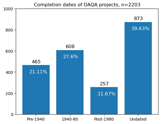
Below are some temporal statistics about completed projects in the DAQA dataset. We divide the data into four periods: before 1940, between 1940-1980, post 1980, and undated. Proportions are calculated as a percentage of the total number of completed projects in the dataset.
Show code cell source
# store all rows with date_start in coverage_range
completion_dates_dict = {'Pre-1940': 0, '1940-80': 0, 'Post-1980': 0, 'Undated': 0}
projects_1940_80 = []
projects_1940_80_firms_dict = dict()
firms_with_projects_1940_80 = []
person_with_projects_1940_80 = []
resource_with_projects_1940_80 = []

for idx,row in daqa_work.iterrows():
    if isinstance(row['coverage_range'], str):
        if "date_end" in row['coverage_range']:
            comp_yr = pd.json_normalize(ast.literal_eval(row['coverage_range'])['date_range'])['date_end.year'].values[0]
            # add counter for comp_yr to dict
            if int(comp_yr) < 1940: completion_dates_dict['Pre-1940'] += 1
            elif int(comp_yr) >= 1940 and int(comp_yr) <= 1980:
                completion_dates_dict['1940-80'] += 1
                projects_1940_80.append(row['_id'])

                # add related firm to list
                if isinstance(row['related_organizations'], str):
                    related_firm = pd.json_normalize(ast.literal_eval(row['related_organizations']))['subject.ori_id'].values[0]
                    firms_with_projects_1940_80.append(related_firm)
                    projects_1940_80_firms_dict[row['_id']] = related_firm

                # add related person to list
                if isinstance(row['related_people'], str):
                    related_person = pd.json_normalize(ast.literal_eval(row['related_people']))['subject.ori_id'].values[0]
                    person_with_projects_1940_80.append(related_person)

                # add related firm to list
                if isinstance(row['related_resources'], str):
                    related_resource = pd.json_normalize(ast.literal_eval(row['related_resources']))['object.ori_id'].values[0]
                    resource_with_projects_1940_80.append(related_resource)

            elif int(comp_yr) > 1980: completion_dates_dict['Post-1980'] += 1
        else:
            completion_dates_dict['Undated'] += 1

# number of projects in DAQA
print('\nThere are {} projects in DAQA.'.format(count_projects))

# number of pre-1940 projects
print('There are {} ({}%) projects with completion dates before 1940.'.\
      format(completion_dates_dict['Pre-1940'], round((completion_dates_dict['Pre-1940']/count_projects)*100,2)))

# number of 1940-1980 projects
print('There are {} ({}%) projects with completion dates between 1940 and 1980.'.\
      format(completion_dates_dict['1940-80'], round((completion_dates_dict['1940-80']/count_projects)*100,2)))

# number of post-1980 projects
print('There are {} ({}%) projects with completion dates after 1980.'.\
      format(completion_dates_dict['Post-1980'], round((completion_dates_dict['Post-1980']/count_projects)*100,2)))

# number of undated projects
print('There are {} ({}%) projects with no completion dates.'\
      .format(completion_dates_dict['Undated'], round((completion_dates_dict['Undated']/count_projects)*100,2)))

print('\n')

# plot completion_dates_dict as a bar chart
plt.bar(range(len(completion_dates_dict)), list(completion_dates_dict.values()), align='center')
plt.xticks(range(len(completion_dates_dict)), list(completion_dates_dict.keys()))
plt.title('Completion dates of DAQA projects, n=2203')

# add labels to bars with propotion in white inside top of bar
for i, v in enumerate(completion_dates_dict.values()):
    plt.text(i - 0.125, v + 20, str(v), size=12)
    plt.text(i - 0.2, v - 75, str(round((v/count_projects)*100,2)) + '%', color='white', size=12)

# make y axis start at 0
plt.ylim(0, 1000)
plt.show()
There are 2203 projects in DAQA.
There are 465 (21.11%) projects with completion dates before 1940.
There are 608 (27.6%) projects with completion dates between 1940 and 1980.
There are 257 (11.67%) projects with completion dates after 1980.
There are 873 (39.63%) projects with no completion dates.
High-level summary of DAQA entities between 1940-1980#
We are particularly interested in data between 1940-1980. Similar to what we generated for the whole dataset, we output high-level statistics for data related to projects in this 1940-1980 period.
Show code cell source
# architects
# filter data accordingly
daqapersons_1940_80 = daqa_persons[daqa_persons['ori_id'].astype(int).isin(person_with_projects_1940_80)].copy()
print('Total number of persons with a related project between 1940-1980:', daqapersons_1940_80.shape[0])
architect_count = daqapersons_1940_80['longterm_roles'].value_counts().reset_index()
architect_count['Proportion'] = round(architect_count['longterm_roles']/architect_count['longterm_roles'].sum(),3)
architect_count['Type'] = np.where(architect_count['index'].str.contains('non-architect'), 'non-architect', 'architect')
display(architect_count\
        .groupby('Type')\
        .sum()\
        .reset_index()\
        .rename(columns={'longterm_roles':'Frequency'})\
        .set_index('Type')
        .sort_values('Frequency', ascending=False))

# firms
# filter data accordingly
daqaorgs_1940_80 = daqa_orgs[daqa_orgs['ori_id'].astype(int).isin(firms_with_projects_1940_80)].copy()
print('\nTotal number of organisations with a related project between 1940-1980:', daqaorgs_1940_80.shape[0])
firm_count = daqaorgs_1940_80['_class_ori'].value_counts().reset_index()
firm_count['Proportion'] = round(firm_count['_class_ori']/firm_count['_class_ori'].sum(),3)
display(firm_count\
        .groupby('index')\
        .sum()\
        .reset_index()\
        .rename(columns={'index':'Type', '_class_ori':'Frequency'})\
        .set_index('Type')
        .sort_values('Frequency', ascending=False))

# projects
# filter data accordingly
daqawork_1940_80 = daqa_work[daqa_work['_id'].isin(projects_1940_80)].copy()
print('\nTotal number of works between 1940-1980 i.e, projects:', daqawork_1940_80.shape[0])
project_count = daqawork_1940_80['_class_ori'].value_counts().reset_index()
project_count['Proportion'] = round(project_count['_class_ori']/project_count['_class_ori'].sum(),3)
display(project_count\
        .groupby('index')\
        .sum()\
        .reset_index()\
        .rename(columns={'index':'Type', '_class_ori':'Frequency'})\
        .set_index('Type')
        .sort_values('Frequency', ascending=False))

# articles
# filter data accordingly
daqaresources_1940_80 = daqa_resources[daqa_resources['ori_id'].astype(int).isin(resource_with_projects_1940_80)].copy()
print('\nTotal number of resources with a related project between 1940-1980 i.e., articles, interviews:', daqaresources_1940_80.shape[0])
article_count = daqaresources_1940_80['_class_ori'].value_counts().reset_index()
article_count['Proportion'] = round(article_count['_class_ori']/article_count['_class_ori'].sum(),3)
display(article_count\
        .groupby('index')\
        .sum()\
        .reset_index()\
        .rename(columns={'index':'Type', '_class_ori':'Frequency'})\
        .set_index('Type')
        .sort_values('Frequency', ascending=False))
Total number of persons with a related project between 1940-1980: 113
| Frequency | Proportion | |
|---|---|---|
| Type | ||
| architect | 112 | 0.991 |
| non-architect | 1 | 0.009 |
Total number of organisations with a related project between 1940-1980: 101
| Frequency | Proportion | |
|---|---|---|
| Type | ||
| "firm" | 101 | 1.0 |
Total number of works between 1940-1980 i.e, projects: 608
| Frequency | Proportion | |
|---|---|---|
| Type | ||
| "structure" | 608 | 1.0 |
Total number of resources with a related project between 1940-1980 i.e., articles, interviews: 471
| Frequency | Proportion | |
|---|---|---|
| Type | ||
| "Photograph" | 288 | 0.611 |
| "LineDrawing" | 67 | 0.142 |
| "Image" | 62 | 0.132 |
| "article" | 47 | 0.100 |
| "interview" | 3 | 0.006 |
| "Portrait" | 2 | 0.004 |
| "publication" | 2 | 0.004 |
Show code cell source
relations_1940_1980 = []
for this_df in [daqapersons_1940_80,daqaorgs_1940_80,daqawork_1940_80,daqaresources_1940_80]:
    for idx,row in this_df.iterrows():
        for col in relationship_cols:
            try:
                if isinstance(row[col], str): relations_1940_1980.append(pd.json_normalize(ast.literal_eval(row[col])))
            except: continue

relations_1940_1980 = pd.concat(relations_1940_1980)
relations_1940_1980 = relations_1940_1980.drop_duplicates()

relations_1940_1980['subject.ori_id'] = relations_1940_1980['subject.ori_id'].astype(str)
relations_1940_1980['object.ori_id'] = relations_1940_1980['object.ori_id'].astype(str)

relations_1940_1980['subject._class_ori'] = np.where(relations_1940_1980['subject._class'] == 'person',
                                       relations_1940_1980['subject.ori_id'].map(arch_nonarch_dict),
                                       relations_1940_1980['subject._class_ori'])
relations_1940_1980['object._class_ori'] = np.where(relations_1940_1980['object._class'] == 'person',
                                       relations_1940_1980['object.ori_id'].map(arch_nonarch_dict),
                                       relations_1940_1980['object._class_ori'])

# relations
print('Total number of relationships for entities related to 1940-1980 works:', relations_1940_1980.shape[0])
display(relations_1940_1980.relation_class.value_counts()\
        .reset_index()\
        .rename(columns={'index':'relation_class','relation_class':'Frequency'})\
        .assign(Proportion = lambda x: round(x['Frequency']/x['Frequency'].sum(),3))\
        .set_index('relation_class')
        .sort_values('Frequency', ascending=False))

# predicate terms
print('\nTotal number of unique predicates for entities related to 1940-1980 works:', relations_1940_1980['predicate.term'].nunique())
display(relations_1940_1980['predicate.term'].value_counts()\
        .reset_index()\
        .rename(columns={'index':'predicate.term','predicate.term':'Frequency'})\
        .assign(Proportion = lambda x: round(x['Frequency']/x['Frequency'].sum(),3))\
        .set_index('predicate.term')
        .sort_values('Frequency', ascending=False))
Total number of relationships for entities related to 1940-1980 works: 8399
| Frequency | Proportion | |
|---|---|---|
| relation_class | ||
| Work_RelatedResource | 2017 | 0.240 |
| Person_RelatedWork | 1472 | 0.175 |
| Person_RelatedPerson | 1218 | 0.145 |
| Organization_RelatedWork | 1091 | 0.130 |
| Person_RelatedOrganization | 903 | 0.108 |
| Work_RelatedPlace | 580 | 0.069 |
| Person_RelatedResource | 293 | 0.035 |
| Resource_RelatedPerson | 253 | 0.030 |
| Organization_RelatedOrganization | 183 | 0.022 |
| Work_RelatedOrganization | 168 | 0.020 |
| Resource_RelatedResource | 49 | 0.006 |
| Organization_RelatedResource | 43 | 0.005 |
| Resource_RelatedOrganization | 43 | 0.005 |
| Resource_RelatedWork | 38 | 0.005 |
| Person_RelatedRecognition | 22 | 0.003 |
| Work_RelatedPerson | 15 | 0.002 |
| Organization_RelatedPerson | 5 | 0.001 |
| Resource_RelatedRecognition | 3 | 0.000 |
| Resource_RelatedPlace | 2 | 0.000 |
| Person_RelatedPlace | 1 | 0.000 |
Total number of unique predicates for entities related to 1940-1980 works: 32
| Frequency | Proportion | |
|---|---|---|
| predicate.term | ||
| WorkedOn | 2303 | 0.274 |
| HasMedia | 2288 | 0.272 |
| Employment | 760 | 0.090 |
| Reference | 602 | 0.072 |
| LocatedIn | 580 | 0.069 |
| RelatedTo | 436 | 0.052 |
| TaughtBy | 245 | 0.029 |
| WorkedWith | 230 | 0.027 |
| InfluencedBy | 160 | 0.019 |
| StudiedWith | 110 | 0.013 |
| KnewSocially | 104 | 0.012 |
| PrecededBy | 93 | 0.011 |
| succeededby | 86 | 0.010 |
| KnewProfessionally | 85 | 0.010 |
| StudiedAt | 57 | 0.007 |
| PartnerOf | 54 | 0.006 |
| IsInvolvedIn | 40 | 0.005 |
| DesignedBy | 38 | 0.005 |
| KnewOf | 30 | 0.004 |
| CollaboratedWith | 19 | 0.002 |
| TravelledTo | 15 | 0.002 |
| ClientOf | 11 | 0.001 |
| WasInfluenceBy | 11 | 0.001 |
| MentoredBy | 10 | 0.001 |
| Founded | 7 | 0.001 |
| Became | 6 | 0.001 |
| Awarded | 5 | 0.001 |
| Read | 4 | 0.000 |
| Attended | 3 | 0.000 |
| TaughtAt | 3 | 0.000 |
| MergedWith | 2 | 0.000 |
| DoneIn | 2 | 0.000 |
Show code cell source
print('###################### PERSON RELATIONSHIPS ######################')
print('\n')
fetch_relation_details(['Person_RelatedWork','Work_RelatedPerson'], relations=relations_1940_1980)
print('\n')
fetch_relation_details(['Person_RelatedPerson'], relations=relations_1940_1980)
print('\n')
fetch_relation_details(['Person_RelatedOrganization','Organization_RelatedPerson'], relations=relations_1940_1980)
print('\n')
fetch_relation_details(['Person_RelatedResource','Resource_RelatedPerson'], relations=relations_1940_1980)
print('\n')
fetch_relation_details(['Person_RelatedRecognition'], relations=relations_1940_1980)
print('\n')
fetch_relation_details(['Person_RelatedPlace'], relations=relations_1940_1980)
print('\n')

print('###################### WORK RELATIONSHIPS ######################')
print('\n')
fetch_relation_details(['Work_RelatedResource','Resource_RelatedWork'], relations=relations_1940_1980)
print('\n')
fetch_relation_details(['Work_RelatedPlace'], relations=relations_1940_1980)
print('\n')
fetch_relation_details(['Work_RelatedRecognition'], relations=relations_1940_1980)
print('\n')

print('###################### ORGANISATION RELATIONSHIPS ######################')
print('\n')
fetch_relation_details(['Organization_RelatedWork','Work_RelatedOrganization'], relations=relations_1940_1980)
print('\n')
fetch_relation_details(['Organization_RelatedOrganization'], relations=relations_1940_1980)
print('\n')
fetch_relation_details(['Recognition_RelatedOrganization'])

print('###################### RESOURCE RELATIONSHIPS ######################')
print('\n')
fetch_relation_details(['Resource_RelatedResource'], relations=relations_1940_1980)
print('\n')
fetch_relation_details(['Resource_RelatedOrganization','Organization_RelatedResource'], relations=relations_1940_1980)
print('\n')
fetch_relation_details(['Resource_RelatedPlace'], relations=relations_1940_1980)
print('\n')
fetch_relation_details(['Resource_RelatedRecognition'], relations=relations_1940_1980)
print('\n')
###################### PERSON RELATIONSHIPS ######################


Total number of Person-Work relations: 1487
| subject._class_ori | object._class_ori | predicate.term | Frequency | |
|---|---|---|---|---|
| 0 | architect | structure | WorkedOn | 1352 |
| 1 | architect | structure | Reference | 86 |
| 2 | architect | structure | InfluencedBy | 16 |
| 3 | structure | architect | DesignedBy | 14 |
| 4 | architect | structure | StudiedAt | 4 |
| 5 | architect | structure | Employment | 3 |
| 6 | architect | structure | TravelledTo | 3 |
| 7 | architect | structure | Attended | 2 |
| 8 | architect | structure | TaughtAt | 2 |
| 9 | non-architect | structure | Reference | 2 |
| 10 | architect | structure | ClientOf | 1 |
| 11 | architect | structure | KnewOf | 1 |
| 12 | structure | architect | ClientOf | 1 |
Total number of Person-Person relations: 1218
| subject._class_ori | object._class_ori | predicate.term | Frequency | |
|---|---|---|---|---|
| 0 | architect | architect | TaughtBy | 232 |
| 1 | architect | architect | WorkedWith | 209 |
| 2 | architect | architect | Reference | 180 |
| 3 | architect | architect | InfluencedBy | 127 |
| 4 | architect | architect | StudiedWith | 100 |
| 5 | architect | architect | KnewSocially | 99 |
| 6 | architect | architect | Employment | 84 |
| 7 | architect | architect | KnewProfessionally | 71 |
| 8 | architect | architect | KnewOf | 26 |
| 9 | architect | non-architect | KnewProfessionally | 13 |
| 10 | architect | architect | MentoredBy | 10 |
| 11 | architect | architect | WasInfluenceBy | 9 |
| 13 | architect | non-architect | StudiedWith | 8 |
| 12 | architect | non-architect | Reference | 8 |
| 14 | architect | architect | CollaboratedWith | 5 |
| 15 | architect | architect | PartnerOf | 5 |
| 16 | architect | non-architect | KnewSocially | 5 |
| 17 | architect | non-architect | CollaboratedWith | 4 |
| 18 | architect | non-architect | WorkedWith | 4 |
| 19 | non-architect | architect | ClientOf | 4 |
| 20 | architect | non-architect | TaughtBy | 3 |
| 21 | architect | architect | ClientOf | 3 |
| 22 | architect | non-architect | InfluencedBy | 3 |
| 23 | architect | non-architect | Employment | 2 |
| 24 | architect | architect | RelatedTo | 2 |
| 25 | non-architect | architect | Employment | 1 |
| 26 | non-architect | architect | Reference | 1 |
Total number of Person-Organization relations: 908
| subject._class_ori | object._class_ori | predicate.term | Frequency | |
|---|---|---|---|---|
| 0 | architect | firm | Employment | 652 |
| 1 | architect | education | StudiedAt | 53 |
| 2 | architect | firm | Reference | 49 |
| 3 | architect | firm | PartnerOf | 49 |
| 4 | architect | education | Employment | 15 |
| 5 | architect | firm | InfluencedBy | 11 |
| 6 | architect | firm | WorkedWith | 11 |
| 7 | architect | firm | TaughtBy | 10 |
| 8 | architect | firm | Founded | 7 |
| 9 | architect | firm | CollaboratedWith | 6 |
| 10 | architect | education | Reference | 5 |
| 11 | architect | education | Read | 3 |
| 12 | architect | education | InfluencedBy | 3 |
| 13 | architect | organisation | Became | 3 |
| 14 | architect | government | WorkedWith | 3 |
| 20 | architect | firm | StudiedWith | 2 |
| 19 | non-architect | firm | Reference | 2 |
| 18 | architect | organisation | Reference | 2 |
| 17 | firm | architect | KnewOf | 2 |
| 15 | architect | organisation | WorkedWith | 2 |
| 16 | architect | organisation | Employment | 2 |
| 29 | architect | firm | WasInfluenceBy | 1 |
| 35 | architect | education | ClientOf | 1 |
| 34 | architect | firm | KnewProfessionally | 1 |
| 33 | architect | organisation | Attended | 1 |
| 32 | architect | firm | KnewOf | 1 |
| 31 | architect | organisation | CollaboratedWith | 1 |
| 30 | architect | education | WorkedOn | 1 |
| 27 | architect | education | TaughtAt | 1 |
| 28 | architect | education | TravelledTo | 1 |
| 26 | firm | architect | Became | 1 |
| 25 | firm | architect | ClientOf | 1 |
| 24 | architect | education | CollaboratedWith | 1 |
| 23 | firm | architect | MergedWith | 1 |
| 22 | non-architect | firm | Employment | 1 |
| 21 | architect | organisation | RelatedTo | 1 |
| 36 | architect | education | Awarded | 1 |
Total number of Person-Resource relations: 546
| subject._class_ori | object._class_ori | predicate.term | Frequency | |
|---|---|---|---|---|
| 0 | interview | architect | Reference | 176 |
| 1 | architect | Photograph | HasMedia | 107 |
| 2 | interview | architect | RelatedTo | 57 |
| 3 | architect | interview | RelatedTo | 55 |
| 4 | architect | Image | HasMedia | 49 |
| 5 | architect | interview | IsInvolvedIn | 39 |
| 6 | architect | Portrait | HasMedia | 23 |
| 7 | interview | non-architect | RelatedTo | 18 |
| 8 | non-architect | interview | RelatedTo | 18 |
| 9 | interview | non-architect | Reference | 2 |
| 10 | architect | publication | Reference | 1 |
| 11 | non-architect | interview | IsInvolvedIn | 1 |
Total number of Person-Recognition relations: 22
| subject._class_ori | object._class_ori | predicate.term | Frequency | |
|---|---|---|---|---|
| 0 | architect | award | TravelledTo | 10 |
| 1 | architect | award | Awarded | 4 |
| 2 | architect | award | Reference | 4 |
| 3 | architect | award | Became | 2 |
| 4 | architect | award | Read | 1 |
| 5 | architect | award | WasInfluenceBy | 1 |
Total number of Person-Place relations: 1
| subject._class_ori | object._class_ori | predicate.term | Frequency | |
|---|---|---|---|---|
| 0 | architect | place | TravelledTo | 1 |
###################### WORK RELATIONSHIPS ######################


Total number of Work-Resource relations: 2055
| subject._class_ori | object._class_ori | predicate.term | Frequency | |
|---|---|---|---|---|
| 0 | structure | Photograph | HasMedia | 1477 |
| 1 | structure | LineDrawing | HasMedia | 397 |
| 2 | structure | Image | HasMedia | 141 |
| 3 | interview | structure | Reference | 38 |
| 4 | structure | Portrait | HasMedia | 2 |
Total number of Work-Place relations: 580
| subject._class_ori | object._class_ori | predicate.term | Frequency | |
|---|---|---|---|---|
| 0 | structure | place | LocatedIn | 580 |
Total number of Work-Recognition relations: 0
| subject._class_ori | object._class_ori | predicate.term | Frequency |
|---|
###################### ORGANISATION RELATIONSHIPS ######################


Total number of Organization-Work relations: 1259
| subject._class_ori | object._class_ori | predicate.term | Frequency | |
|---|---|---|---|---|
| 0 | firm | structure | WorkedOn | 950 |
| 1 | structure | firm | RelatedTo | 144 |
| 2 | firm | structure | RelatedTo | 141 |
| 3 | structure | firm | DesignedBy | 24 |
Total number of Organization-Organization relations: 183
| subject._class_ori | object._class_ori | predicate.term | Frequency | |
|---|---|---|---|---|
| 0 | firm | firm | PrecededBy | 93 |
| 1 | firm | firm | succeededby | 86 |
| 2 | firm | firm | CollaboratedWith | 2 |
| 3 | firm | firm | MergedWith | 1 |
| 4 | firm | firm | WorkedWith | 1 |
Total number of Recognition-Organization relations: 1
| subject._class_ori | object._class_ori | predicate.term | Frequency | |
|---|---|---|---|---|
| 0 | award | education | StudiedAt | 1 |
###################### RESOURCE RELATIONSHIPS ######################


Total number of Resource-Resource relations: 49
| subject._class_ori | object._class_ori | predicate.term | Frequency | |
|---|---|---|---|---|
| 0 | article | Article | HasMedia | 36 |
| 1 | interview | Audio | HasMedia | 6 |
| 2 | interview | Transcript | HasMedia | 5 |
| 3 | interview | Youtube | HasMedia | 2 |
Total number of Resource-Organization relations: 86
| subject._class_ori | object._class_ori | predicate.term | Frequency | |
|---|---|---|---|---|
| 0 | interview | firm | Reference | 41 |
| 1 | firm | Photograph | HasMedia | 31 |
| 2 | firm | Portrait | HasMedia | 9 |
| 3 | firm | LineDrawing | HasMedia | 2 |
| 4 | firm | Image | HasMedia | 1 |
| 5 | interview | education | Reference | 1 |
| 6 | interview | organisation | Reference | 1 |
Total number of Resource-Place relations: 2
| subject._class_ori | object._class_ori | predicate.term | Frequency | |
|---|---|---|---|---|
| 0 | interview | place | DoneIn | 2 |
Total number of Resource-Recognition relations: 3
| subject._class_ori | object._class_ori | predicate.term | Frequency | |
|---|---|---|---|---|
| 0 | interview | award | Reference | 3 |
1940-1980 projects and firms#
Below are some statistics about project characteristics and firms in the DAQA dataset of only projected completed between 1940 and 1980. Proportions under the 1940-1980 PROJECTS subheading are calculated as a percentage of the total number of projects completed between 1940 and 1980 in the dataset. Proportions under the 1940-1980 FIRMS subheading are calculated as a percentage of the total number of firms related to projects completed between 1940 and 1980 in the dataset.
We define an extant project as one that has a populated
is_demolishedfield and the value isFalseWe define a demolished project as one that has a populated
is_demolishedfield and the value isTrue
Show code cell source
print('###################### 1940-1980 PROJECTS ######################')

# filter data accordingly
daqawork_1940_80 = daqa_work[daqa_work['_id'].isin(projects_1940_80)].copy()

print('\nQ: How many projects are recorded in DAQA between 1940-1980?')
count_projects = len(daqawork_1940_80)
print(f'A: There are {count_projects} projects between 1940-1980.')

# we define a extant buiulding where "is_demolished" field is False
print('\nQ: what % of projects completed in 1940-1980 are extant?')
count_projects_extant = len(daqawork_1940_80[daqawork_1940_80['is_demolished'] == False])
prop_projects_extant = round((count_projects_extant / count_projects) * 100, 2)
print(f'A: {prop_projects_extant}% ({count_projects_extant}) of DAQA projects between 1940-1980 are extant.')

# we define a extant buiulding where "is_demolished" field is True
print('\nQ: what % of projects completed in 1940-1980 are demolished?')
count_projects_demolished = len(daqawork_1940_80[daqawork_1940_80['is_demolished'] == True])
prop_projects_demolished = round((count_projects_demolished / count_projects) * 100, 2)
print(f'A: {prop_projects_demolished}% ({count_projects_demolished}) of DAQA projects between 1940-1980 are demolished.')

print('\n*It should be noted that there are 5 DAQA projects between 1940-1980 with missing demolished information.')

# we define a project with an address as one that has a populated "address" field
print('\nQ: what % of projects between 1940-1980 have addresses?')
count_projects_with_address = len(daqawork_1940_80[daqawork_1940_80.coverage_range.apply(lambda x: "address" in x)])
prop_projects_with_address = round((count_projects_with_address / count_projects) * 100, 2)
print(f'A: {prop_projects_with_address}% ({count_projects_with_address}) of DAQA projects between 1940-1980 have addresses.')

# we define a project with a geocode date as one that has a populated "longitude" field
print('\nQ: what % of projects between 1940-1980 have geocodes (lat/long)?')
count_projects_with_geocodes = len(daqawork_1940_80[daqawork_1940_80.coverage_range.apply(lambda x: "latitude" in x)])
prop_projects_with_geocodes = round((count_projects_with_geocodes / count_projects) * 100, 2)
print(f'A: {prop_projects_with_geocodes}% ({count_projects_with_geocodes}) of DAQA projects between 1940-1980 have geocodes.')

# we define a project with an associated firm as one that has a populated "related_organizations" field
print('\nQ: how many projects between 1940-1980 have associated firms?')
daqawork_1940_80_firms = daqawork_1940_80[daqawork_1940_80.related_organizations.notnull()]
count_projects_with_firms = len(daqawork_1940_80_firms)
prop_projects_with_firms = round((count_projects_with_firms / count_projects) * 100, 2)
print(f'A: {prop_projects_with_firms}% ({count_projects_with_firms}) of DAQA projects between 1940-1980 have associated firms.')

# we define a project with no associated architects as one that has no populated "related_people" field
print('\nQ: what % of projects between 1940-1980 have associated firms but no architects?')
count_projects_with_firms_no_architects = len(daqawork_1940_80[(daqawork_1940_80.related_organizations.notnull()) &\
                                                        (daqawork_1940_80.related_people.isnull())])
prop_projects_with_firms_no_architects = round((count_projects_with_firms_no_architects / count_projects) * 100, 2)
print(f'A: {prop_projects_with_firms_no_architects}% ({count_projects_with_firms_no_architects}) of DAQA projects between 1940-1980 have associated firms but no architects.')

# we define a project with an associated architect as one that has a populated "related_people" field
print('\nQ: how many projects between 1940-1980 have associated architects?')
count_projects_with_architects = len(daqawork_1940_80[daqawork_1940_80.related_people.notnull()])
prop_projects_with_architects = round((count_projects_with_architects / count_projects) * 100, 2)
print(f'A: {prop_projects_with_architects}% ({count_projects_with_architects}) of DAQA projects between 1940-1980 have associated architects.')

# we define a project with an associated architects as one that has a populated "related people" field
# and we define a project with no associated firms as one that has a no populated "related organizations" field
print('\nQ: what % of projects between 1940-1980 have associated architects but no firms?')
count_projects_with_architects_no_firms = len(daqawork_1940_80[(daqawork_1940_80.related_organizations.isnull()) &\
                                                        (daqawork_1940_80.related_people.notnull())])
prop_projects_with_architects_no_firms = round((count_projects_with_architects_no_firms / count_projects) * 100, 2)
print(f'A: {prop_projects_with_architects_no_firms}% ({count_projects_with_architects_no_firms}) of DAQA projects between 1940-1980 have associated architects but no firms.')


print('\n###################### 1940-1980 FIRMS ######################')

# filter data accordingly
daqafirms_1940_80 = daqa_firms[daqa_firms['ori_id'].astype(int).isin(firms_with_projects_1940_80)].copy()

print('\nQ: How many firms are recorded in DAQA between 1940-1980?')
count_firms = len(daqafirms_1940_80)
print(f'A: There are {count_firms} firms between 1940-1980.')

# we define an operating firm as an organisation that has a populated "operation" field with a start date
print('\nQ: what % of firms between 1940-1980 have ‘operating years’ recorded (just start)?')
count_firms_with_operating_start = len(daqafirms_1940_80[daqafirms_1940_80.operation.apply(lambda x: "date_start" in x if isinstance(x, str) else False)])
prop_firms_with_operating_start = round((count_firms_with_operating_start / count_firms) * 100, 2)
print(f'A: {prop_firms_with_operating_start}% ({count_firms_with_operating_start}) of DAQA firms between 1940-1980 have operating years recorded (just start).')

# we define an operating firm as an organisation that has a populated "operation" field with start and end dates
print('\nQ: what % of firms between 1940-1980 have ‘operating years’ recorded (start and end)?')
count_firms_with_operating_years = len(daqafirms_1940_80[daqafirms_1940_80.operation.apply(lambda x: ("date_start" in x) & ("date_end" in x) if isinstance(x, str) else False)])
prop_firms_with_operating_years = round((count_firms_with_operating_years / count_firms) * 100, 2)
print(f'A: {prop_firms_with_operating_years}% ({count_firms_with_operating_years}) of DAQA firms between 1940-1980 have operating years recorded (start and end).')
###################### 1940-1980 PROJECTS ######################

Q: How many projects are recorded in DAQA between 1940-1980?
A: There are 608 projects between 1940-1980.

Q: what % of projects completed in 1940-1980 are extant?
A: 86.84% (528) of DAQA projects between 1940-1980 are extant.

Q: what % of projects completed in 1940-1980 are demolished?
A: 12.34% (75) of DAQA projects between 1940-1980 are demolished.

*It should be noted that there are 5 DAQA projects between 1940-1980 with missing demolished information.

Q: what % of projects between 1940-1980 have addresses?
A: 96.05% (584) of DAQA projects between 1940-1980 have addresses.

Q: what % of projects between 1940-1980 have geocodes (lat/long)?
A: 85.86% (522) of DAQA projects between 1940-1980 have geocodes.

Q: how many projects between 1940-1980 have associated firms?
A: 78.29% (476) of DAQA projects between 1940-1980 have associated firms.

Q: what % of projects between 1940-1980 have associated firms but no architects?
A: 16.94% (103) of DAQA projects between 1940-1980 have associated firms but no architects.

Q: how many projects between 1940-1980 have associated architects?
A: 82.07% (499) of DAQA projects between 1940-1980 have associated architects.

Q: what % of projects between 1940-1980 have associated architects but no firms?
A: 20.72% (126) of DAQA projects between 1940-1980 have associated architects but no firms.

###################### 1940-1980 FIRMS ######################

Q: How many firms are recorded in DAQA between 1940-1980?
A: There are 101 firms between 1940-1980.

Q: what % of firms between 1940-1980 have ‘operating years’ recorded (just start)?
A: 81.19% (82) of DAQA firms between 1940-1980 have operating years recorded (just start).

Q: what % of firms between 1940-1980 have ‘operating years’ recorded (start and end)?
A: 67.33% (68) of DAQA firms between 1940-1980 have operating years recorded (start and end).
Education#
Below are some education qualification characteristics of people records in the DAQA dataset. Proportions are calculated as a percentage of the total number of people in the dataset.
We focus on the data of four universities: UQ, BCTC, QIT, and QUT. The latter three also grouped together, and represented as BCTC/QIT/QUT. We compute statistics for each university separately and then visualise the data for UQ and BCTC/QIT/QUT.
We define a person with a education data as one that has a populated
education_trainingsfieldWe define a person with a education year data as one that has a populated
date_endfield in theeducation_trainingsfield
Show code cell source
# load data
daqa_persons = df_daqa_dict['person']
daqa_persons_with_education_data = daqa_persons[daqa_persons['education_trainings'].notnull()].copy()

print('\nQ: How many persons are recorded in DAQA?')
count_persons = len(daqa_persons)
print(f'A: There are {count_persons} people in DAQA.')

# we define a person with a education data as one that has a populated "education_trainings" field
print('\nQ: what % of people have education data?')
count_persons_with_education_data = len(daqa_persons_with_education_data)
prop_persons_with_education_data = round((count_persons_with_education_data / count_persons) * 100, 2)
print(f'A: {prop_persons_with_education_data}% ({count_persons_with_education_data}) of people with education data.')

# we define a person with a education year data as one that has a populated "date_end" field in the "education_trainings" field
print('\nQ: what % of people have education data (with years)?')
daqa_persons_with_education_year_data = daqa_persons_with_education_data[daqa_persons_with_education_data\
                                                                         .education_trainings.apply(lambda x: "date_end" in x)]
count_persons_with_education_year_data = len(daqa_persons_with_education_year_data)
prop_persons_with_education_year_data = round((count_persons_with_education_year_data / count_persons) * 100, 2)
print(f'A: {prop_persons_with_education_year_data}% ({count_persons_with_education_year_data}) of people with education year data.')
Q: How many persons are recorded in DAQA?
A: There are 1103 people in DAQA.

Q: what % of people have education data?
A: 20.58% (227) of people with education data.

Q: what % of people have education data (with years)?
A: 17.86% (197) of people with education year data.
Queensland universities#
UQ#
Show code cell source
education_training_df = pd.DataFrame()

for idx, row in daqa_persons_with_education_data.iterrows():
    person_id = row['ori_id']
    education_training_data = pd.json_normalize(ast.literal_eval(row['education_trainings']))
    education_training_data['ori_id'] = person_id
    education_training_df = education_training_df.append(education_training_data)

# remove erroneous row
education_training_df = education_training_df[~education_training_df['organization.name'].str.contains('note: interview UQ',na=False)]

def print_filtered_data(df, filter, display_output=True):
    filtered_df = df[df['organization.name'].str.contains('|'.join(filter),na=False)]
    if display_output:
        display(filtered_df['organization.name']\
                .value_counts()\
                .reset_index()\
                .rename(columns={'index': 'organization',
                                'organization.name': 'count'}))
    return filtered_df.shape[0]

print('\nQ: How many education records from UQ exist in DAQA?')
filterd_count_uq = print_filtered_data(education_training_df, ['UQ'])
print('A: There are {} education records with from UQ.'.format(filterd_count_uq))
Q: How many education records from UQ exist in DAQA?
| organization | count | |
|---|---|---|
| 0 | UQ | 99 |
| 1 | BCTC/UQ | 11 |
| 2 | QUT, UQ | 1 |
| 3 | BCTC?UQ | 1 |
A: There are 112 education records with from UQ.
BCTC#
Show code cell source
print('Q: How many people have education data from BCTC?')
filterd_count_bctc = print_filtered_data(education_training_df, ['BCTC','BRISBANE'])
print('A: There are {} people with education data from BCTC.'.format(filterd_count_bctc))
Q: How many people have education data from BCTC?
| organization | count | |
|---|---|---|
| 0 | BCTC | 42 |
| 1 | BCTC/UQ | 11 |
| 2 | BRISBANE CENTRAL TECHNICAL COLLEGE | 3 |
| 3 | BCTC?UQ | 1 |
A: There are 57 people with education data from BCTC.
QIT#
Show code cell source
print('Q: How many people have education data from QIT?')
filterd_count_qit = print_filtered_data(education_training_df, ['QIT'])
print('A: There are {} people with education data from QIT.'.format(filterd_count_qit))
Q: How many people have education data from QIT?
| organization | count | |
|---|---|---|
| 0 | QIT | 21 |
A: There are 21 people with education data from QIT.
QUT#
Show code cell source
print('Q: How many people have education data from QUT?')
filterd_count_qut = print_filtered_data(education_training_df, ['QUT'])
print('A: There are {} people with education data from QUT.'.format(filterd_count_qut))
Q: How many people have education data from QUT?
| organization | count | |
|---|---|---|
| 0 | QUT | 10 |
| 1 | OHIO_STATE_UNIandQUT | 1 |
| 2 | QUT, UQ | 1 |
A: There are 12 people with education data from QUT.
Visual comparison#
Show code cell source
# create a bar chart with all the filterd_count values
fig, ax = plt.subplots(figsize=(10, 5))
ax.bar(['UQ', 'BCTC', 'QIT', 'QUT'], [filterd_count_uq, filterd_count_bctc, filterd_count_qit, filterd_count_qut])
ax.set_ylabel('Count')
ax.set_title('Count of education records from each institution')
ax.text(0.5, -0.125, 'Note: there are some non-disjoint cases in the data.', size=12, ha="center", transform=ax.transAxes)
for p in ax.patches: ax.annotate(str(p.get_height()), (p.get_x()+.32, p.get_height() + 3), size=15)
ax.set_ylim([0, 130])
plt.show()

# create a bar chart with all the filterd_count values
fig, ax = plt.subplots(figsize=(10, 5))
ax.bar(['UQ', 'BCTC/QIT/QUT'], [filterd_count_uq, filterd_count_bctc + filterd_count_qit + filterd_count_qut])
ax.set_ylabel('Count')
ax.set_title('Count of education records from each institution (combined)')
ax.text(0.5, -0.125, 'Note: there are some non-disjoint cases in the data.', size=12, ha="center", transform=ax.transAxes)
for p in ax.patches: ax.annotate(str(p.get_height()), (p.get_x()+.32, p.get_height() + 3), size=15)
ax.set_ylim([0, 130])
plt.show()
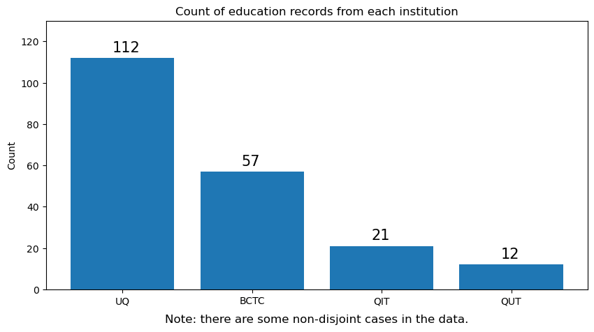
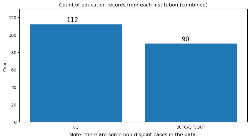
Education by period#
Below are some temporal statistics of education qualification data of people records in the DAQA dataset - but before computing summary statistics the data requires some cleaning. Under the heading DATA QUALITY OF EDUCATION RECORDS, we walk through the applied cleaning steps.
Summary statistics are presented for two periods: before 1940 and between 1940-1980. These outputs can be found under their respective subheadings. Proportions under the 1940-1980 EDUCATION subheading are calculated as a percentage of the total number of people with education records in the dataset during this period. Proportions under the 1940-Present EDUCATION subheading are calculated as a percentage of the total number of people with education records in the dataset during this period.
Show code cell source
print('\n###################### DATA QUALITY OF EDUCATION RECORDS ######################')

education_training_df_with_dates = education_training_df[education_training_df['coverage_range.date_range.date_end.year'].notnull()].copy()

clean_columns_dict = {'organization.name': 'name',
                      'organization.type': 'type',
                      'organization.qualification': 'qual',
                      'coverage_range.place': 'place',
                      'coverage_range.date_range.date_end.year': 'end_year',
                      'ori_id': 'ori_id'}

print('\nFor some records, the data is messy in terms of the end year for a corresponding education record.')
print('\nBelow we provide all the eductional records with unconventional values in the end year field')

check_string_len_cond = (education_training_df_with_dates['coverage_range.date_range.date_end.year'].str.len() > 4)
display(education_training_df_with_dates[check_string_len_cond]\
        .sort_values(by=['organization.name'], ascending=False)\
        .rename(columns=clean_columns_dict))

print('\n1. Remove incomplete records. These records do not hold any temporal information.')
disregard_incomplete_records = (education_training_df_with_dates['coverage_range.date_range.date_end.year'].str.contains('incom', na=False))

display(education_training_df_with_dates[check_string_len_cond & ~disregard_incomplete_records]\
        .sort_values(by=['organization.name'], ascending=False)\
        .rename(columns=clean_columns_dict))

print('\n2. Remove non-numeric suffixal characters such as "?" and "s". As we are interested in a certain period, granularity is not important.')

# remove non-numeric characters such as "?" and "s" for the end year field
education_training_df_with_dates['coverage_range.date_range.date_end.year'] = education_training_df_with_dates['coverage_range.date_range.date_end.year']\
    .str.replace('?', '', regex=False).str.replace('s', '', regex=False)

display(education_training_df_with_dates[check_string_len_cond & ~disregard_incomplete_records]\
        .sort_values(by=['organization.name'], ascending=False)\
        .rename(columns=clean_columns_dict))

print('\n3. Fix the row with two years separated by a comma. Again as we are interested in a certain period, we can temporarily replace this with the most recent year.')

# remove non-numeric characters such as "?" and "s" for the end year field
education_training_df_with_dates['coverage_range.date_range.date_end.year'] = education_training_df_with_dates['coverage_range.date_range.date_end.year']\
    .str.replace('2003, 2008', '2008', regex=False)

display(education_training_df_with_dates[check_string_len_cond & ~disregard_incomplete_records]\
        .sort_values(by=['organization.name'], ascending=False)\
        .rename(columns=clean_columns_dict))
###################### DATA QUALITY OF EDUCATION RECORDS ######################

For some records, the data is messy in terms of the end year for a corresponding education record.

Below we provide all the eductional records with unconventional values in the end year field
| name | type | qual | place | end_year | ori_id | |
|---|---|---|---|---|---|---|
| 0 | UQ | UNI | NaN | QLD | incomplete | 254 |
| 0 | UQ | UNI | BArch | Qld | incomplete | 267 |
| 1 | UQ | UNI | DipArch | QLD | incomplete | 384 |
| 0 | UQ | UNI | DipArch | QLD | 1945? | 376 |
| 0 | UQ | UNI | NaN | QLD | incomplete | 736 |
| 1 | UQ | UNI | BArch | QLD | 1969? | 117 |
| 3 | UNSW | UNI | Archives | NSW | incomplete | 384 |
| 0 | STC | NSW | NaN | Colle | incom | 538 |
| 2 | QUT, UQ | UNI | PhD (hon) | QLD | 2003, 2008 | 174 |
| 0 | QIT | INSTITUTE | CERT | QLD | 1968? | 13 |
| 0 | QIT | INSTITUTE | CERT | QLD | 1968? | 14 |
| 0 | QIT | INSTITUTE | CERT | QLD | 1968? | 10 |
| 0 | QIT | COLLEGE | DipArch | QLD | 1979? | 380 |
| 0 | NANGLE IoT | DISTANCE EDUCATION | DipArch | SYDNEY | 1960s | 355 |
| 0 | Melbourne | UNI | BArch | VIC | 1939? | 349 |
| 1 | Durhan | UNI | Landscape | UK | 1965? | 713 |
| 0 | Budapest | UNI | NaN | Hungary | incomplete | 584 |
| 0 | BCTC | COLLEGE | CertArch | QLD | 1961? | 627 |
| 0 | BCTC | COLLEGE | BArch | QLD | incomplete | 273 |
| 0 | AA | INDEPENDENT | DipArch | UK | 1890? | 636 |
| 0 | NaN | NaN | NaN | Vienna | 1940s | 166 |
| 1 | NaN | UNI | BACHELOR OF ARCHITECTURE | NaN | 1968? | 4 |
1. Remove incomplete records. These records do not hold any temporal information.
| name | type | qual | place | end_year | ori_id | |
|---|---|---|---|---|---|---|
| 0 | UQ | UNI | DipArch | QLD | 1945? | 376 |
| 1 | UQ | UNI | BArch | QLD | 1969? | 117 |
| 2 | QUT, UQ | UNI | PhD (hon) | QLD | 2003, 2008 | 174 |
| 0 | QIT | INSTITUTE | CERT | QLD | 1968? | 13 |
| 0 | QIT | INSTITUTE | CERT | QLD | 1968? | 14 |
| 0 | QIT | INSTITUTE | CERT | QLD | 1968? | 10 |
| 0 | QIT | COLLEGE | DipArch | QLD | 1979? | 380 |
| 0 | NANGLE IoT | DISTANCE EDUCATION | DipArch | SYDNEY | 1960s | 355 |
| 0 | Melbourne | UNI | BArch | VIC | 1939? | 349 |
| 1 | Durhan | UNI | Landscape | UK | 1965? | 713 |
| 0 | BCTC | COLLEGE | CertArch | QLD | 1961? | 627 |
| 0 | AA | INDEPENDENT | DipArch | UK | 1890? | 636 |
| 0 | NaN | NaN | NaN | Vienna | 1940s | 166 |
| 1 | NaN | UNI | BACHELOR OF ARCHITECTURE | NaN | 1968? | 4 |
2. Remove non-numeric suffixal characters such as "?" and "s". As we are interested in a certain period, granularity is not important.
| name | type | qual | place | end_year | ori_id | |
|---|---|---|---|---|---|---|
| 0 | UQ | UNI | DipArch | QLD | 1945 | 376 |
| 1 | UQ | UNI | BArch | QLD | 1969 | 117 |
| 2 | QUT, UQ | UNI | PhD (hon) | QLD | 2003, 2008 | 174 |
| 0 | QIT | INSTITUTE | CERT | QLD | 1968 | 13 |
| 0 | QIT | INSTITUTE | CERT | QLD | 1968 | 14 |
| 0 | QIT | INSTITUTE | CERT | QLD | 1968 | 10 |
| 0 | QIT | COLLEGE | DipArch | QLD | 1979 | 380 |
| 0 | NANGLE IoT | DISTANCE EDUCATION | DipArch | SYDNEY | 1960 | 355 |
| 0 | Melbourne | UNI | BArch | VIC | 1939 | 349 |
| 1 | Durhan | UNI | Landscape | UK | 1965 | 713 |
| 0 | BCTC | COLLEGE | CertArch | QLD | 1961 | 627 |
| 0 | AA | INDEPENDENT | DipArch | UK | 1890 | 636 |
| 0 | NaN | NaN | NaN | Vienna | 1940 | 166 |
| 1 | NaN | UNI | BACHELOR OF ARCHITECTURE | NaN | 1968 | 4 |
3. Fix the row with two years separated by a comma. Again as we are interested in a certain period, we can temporarily replace this with the most recent year.
| name | type | qual | place | end_year | ori_id | |
|---|---|---|---|---|---|---|
| 0 | UQ | UNI | DipArch | QLD | 1945 | 376 |
| 1 | UQ | UNI | BArch | QLD | 1969 | 117 |
| 2 | QUT, UQ | UNI | PhD (hon) | QLD | 2008 | 174 |
| 0 | QIT | INSTITUTE | CERT | QLD | 1968 | 13 |
| 0 | QIT | INSTITUTE | CERT | QLD | 1968 | 14 |
| 0 | QIT | INSTITUTE | CERT | QLD | 1968 | 10 |
| 0 | QIT | COLLEGE | DipArch | QLD | 1979 | 380 |
| 0 | NANGLE IoT | DISTANCE EDUCATION | DipArch | SYDNEY | 1960 | 355 |
| 0 | Melbourne | UNI | BArch | VIC | 1939 | 349 |
| 1 | Durhan | UNI | Landscape | UK | 1965 | 713 |
| 0 | BCTC | COLLEGE | CertArch | QLD | 1961 | 627 |
| 0 | AA | INDEPENDENT | DipArch | UK | 1890 | 636 |
| 0 | NaN | NaN | NaN | Vienna | 1940 | 166 |
| 1 | NaN | UNI | BACHELOR OF ARCHITECTURE | NaN | 1968 | 4 |
Show code cell source
print('\n###################### 1940-1980 EDUCATION ######################')

# clean year data for temporal analysis
education_training_df_with_clean_dates = education_training_df_with_dates[~check_string_len_cond].copy()
education_training_df_with_clean_dates = education_training_df_with_clean_dates\
    .append(education_training_df_with_dates[check_string_len_cond & ~disregard_incomplete_records])

education_training_df_with_clean_dates['coverage_range.date_range.date_end.year'] = education_training_df_with_clean_dates['coverage_range.date_range.date_end.year'].astype(int)

education_training_df_1940_1980 = education_training_df_with_clean_dates[(education_training_df_with_clean_dates['coverage_range.date_range.date_end.year'] >= 1940) & \
                                                                   (education_training_df_with_clean_dates['coverage_range.date_range.date_end.year'] <= 1980)].copy()

print('\nQ: How many education records exist in DAQA between 1940-1980?')
count_ed_records_1940_1980 = len(education_training_df_1940_1980)
print(f'A: There are {count_ed_records_1940_1980} education records between 1940-1980.')

print('\nQ: How many education records exist from UQ between 1940-1980?')
count_ed_records_1940_1980_uq = print_filtered_data(education_training_df_1940_1980, ['UQ'], display_output=False)
prop_ed_records_1940_1980_uq = count_ed_records_1940_1980_uq / count_ed_records_1940_1980
print(f'A: There are {count_ed_records_1940_1980_uq} ({prop_ed_records_1940_1980_uq:.2%}) education records from UQ between 1940-1980.')

print('\nQ: How many education records exist from BCTC/QIT/QIT between 1940-1980?')
count_ed_records_1940_1980_rest = print_filtered_data(education_training_df_1940_1980, ['BCTC', 'QIT', 'QUT','BRISBANE'], display_output=False)
prop_ed_records_1940_1980_rest = count_ed_records_1940_1980_rest / count_ed_records_1940_1980
print(f'A: There are {count_ed_records_1940_1980_rest} ({prop_ed_records_1940_1980_rest:.2%}) education records from BCTC/QIT/QUT between 1940-1980.')


print('\n###################### 1940-Present EDUCATION ######################')

# remove rows with more than 4 characters in string
education_training_df_1940_present = education_training_df_with_clean_dates[(education_training_df_with_clean_dates['coverage_range.date_range.date_end.year'] >= 1940)].copy()

print('\nQ: How many education records exist in DAQA between 1940-Present?')
count_ed_records_1940_present = len(education_training_df_1940_present)
print(f'A: There are {count_ed_records_1940_present} education records between 1940-Present.')

print('\nQ: How many education records exist from UQ between 1940-Present?')
count_ed_records_1940_present_uq = print_filtered_data(education_training_df_1940_present, ['UQ'], display_output=False)
prop_ed_records_1940_present_uq = count_ed_records_1940_present_uq / count_ed_records_1940_present
print(f'A: There are {count_ed_records_1940_present_uq} ({prop_ed_records_1940_present_uq:.2%}) education records from UQ between 1940-Present.')

print('\nQ: How many education records exist from BCTC/QIT/QIT between 1940-Present?')
count_ed_records_1940_present_rest = print_filtered_data(education_training_df_1940_present, ['BCTC', 'QIT', 'QUT','BRISBANE'], display_output=False)
prop_ed_records_1940_present_rest = count_ed_records_1940_present_rest / count_ed_records_1940_present
print(f'A: There are {count_ed_records_1940_present_rest} ({prop_ed_records_1940_present_rest:.2%}) education records from BCTC/QIT/QUT between 1940-Present.')
###################### 1940-1980 EDUCATION ######################

Q: How many education records exist in DAQA between 1940-1980?
A: There are 158 education records between 1940-1980.

Q: How many education records exist from UQ between 1940-1980?
A: There are 83 (52.53%) education records from UQ between 1940-1980.

Q: How many education records exist from BCTC/QIT/QIT between 1940-1980?
A: There are 42 (26.58%) education records from BCTC/QIT/QUT between 1940-1980.

###################### 1940-Present EDUCATION ######################

Q: How many education records exist in DAQA between 1940-Present?
A: There are 193 education records between 1940-Present.

Q: How many education records exist from UQ between 1940-Present?
A: There are 98 (50.78%) education records from UQ between 1940-Present.

Q: How many education records exist from BCTC/QIT/QIT between 1940-Present?
A: There are 57 (29.53%) education records from BCTC/QIT/QUT between 1940-Present.
Persons with related works#
In this section, we explore project activity of people in DAQA. We start by first categorising people into five groups: People with one related work, 2-3 works, 4-10 works, 11-50 works, and +50 works. We then visualise the distribution of these categories. We are particulatly interested in architects with more than 50 related works.
Given the distribution, we also explore the presence of the Pareto principle - in other words, are a majority of completed projects related to only a small number of architects? We plot the cumulative distribution of architects and their related works.
Show code cell source
# load data
daqa_persons_with_related_works = daqa_persons[daqa_persons['related_works'].notnull()].copy()

related_works_raw = pd.DataFrame()
for index, row in daqa_persons_with_related_works.iterrows():
    related_works_raw = related_works_raw.append(pd.json_normalize(ast.literal_eval(row['related_works'])))

# get all person ids with related works
related_works_raw = related_works_raw[['relation_class','subject.ori_id','object.ori_id']].drop_duplicates()

Person_RelatedWork_cond = (related_works_raw['relation_class']=='Person_RelatedWork')
Work_RelatedPerson_cond = (related_works_raw['relation_class']=='Work_RelatedPerson')

person_ids_related_works = related_works_raw[Person_RelatedWork_cond]['subject.ori_id']\
    .value_counts().reset_index().rename(columns={'index': 'id', 'subject.ori_id': 'count'})\
    .append(related_works_raw[Work_RelatedPerson_cond]['object.ori_id']\
            .value_counts().reset_index().rename(columns={'index': 'id', 'object.ori_id': 'count'}))

person_ids_related_works = person_ids_related_works.groupby('id').sum().reset_index()

person_ids_related_works['count_cat'] = np.where((person_ids_related_works['count'] < 2), person_ids_related_works['count'],
                                np.where((person_ids_related_works['count'] <= 3),'2-3',
                                np.where((person_ids_related_works['count'] <= 10),'4-10',
                                np.where((person_ids_related_works['count'] <= 50),'11-50','+50'))))


# plot horizontal bar chart
ax = person_ids_related_works['count_cat'].value_counts().reindex(['1','2-3','4-10','11-50','+50']).sort_values()\
    .plot(kind='barh', figsize=(10,5), title='Number of (unique) Related Works per Person')

# add bar labels with proportions
for p in ax.patches:
    ax.annotate(f'{p.get_width()} ({p.get_width()/len(person_ids_related_works):.2%})', (p.get_width()+1.05, p.get_y()+0.15), size=12)

# increase x-axis
ax.set_xlim(0, 110)

plt.show()

print('\nQ: Who has 50 or more related works?')
person_ids_with_over50works = person_ids_related_works[person_ids_related_works['count_cat']=='+50']['id'].values.tolist()
daqa_persons['ori_id'] = daqa_persons['ori_id'].astype(int)

top_six = pd.merge(daqa_persons[daqa_persons['ori_id'].astype(int).isin(person_ids_with_over50works)][['ori_id','display_name']].rename(columns={'ori_id': 'id'}),
         person_ids_related_works[person_ids_related_works['id'].isin(person_ids_with_over50works)], on='id')

# get person records with 50 or more related works
display(top_six[['display_name','count']].sort_values(by='count', ascending=False))

print('\n###################### PARETO PRINCIPLE ######################')

#check for pareto principle
samples = pd.DataFrame({"Number of projects": person_ids_related_works['count'].sort_values(ascending=False).values})

# Add cumulative percentage column
samples["cum_percentage"] = round(samples["Number of projects"].cumsum()/samples["Number of projects"].sum()*100,2)

# Set figure and axis
fig, ax = plt.subplots(figsize=(10,5))

# Plot bars (i.e. frequencies)
ax.bar(samples.index, samples["Number of projects"])
ax.set_title('Pareto-like distribution')
ax.set_xlabel("Architects (ordered by related work frequency)")
ax.set_ylabel("Frequency")

# Second y axis (i.e. cumulative percentage)
ax2 = ax.twinx()
ax2.plot(samples.index, samples["cum_percentage"], color="red")
ax2.axhline(77, color="orange", linestyle="dashed", alpha=1)
ax2.yaxis.set_major_formatter(PercentFormatter())

# add more ticks to y axis
ax2.set_yticks([0,25,50,75,100])
ax2.set_ylabel("Cumulative Percentage")

# color regions on the x-axis
ax.axvspan(0, 70, alpha=0.05, color='orange')

# add an annotation for the 80% line
ax2.annotate('25% of architects (70)', xy=(0, 100), xytext=(5, 100))
ax2.annotate('77% of completed projects (1628)', xy=(0, 100), xytext=(195, 79))

plt.show()
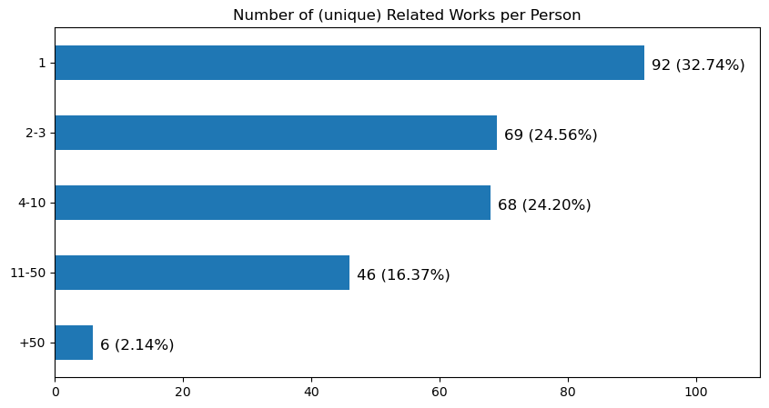
Q: Who has 50 or more related works?
| display_name | count | |
|---|---|---|
| 3 | "Lange Powell" | 145 |
| 5 | "Karl Langer" | 82 |
| 4 | "Graham W. Bligh" | 78 |
| 0 | "Rex Addison" | 75 |
| 1 | "Robin Gibson" | 70 |
| 2 | "John Dalton" | 67 |
###################### PARETO PRINCIPLE ######################
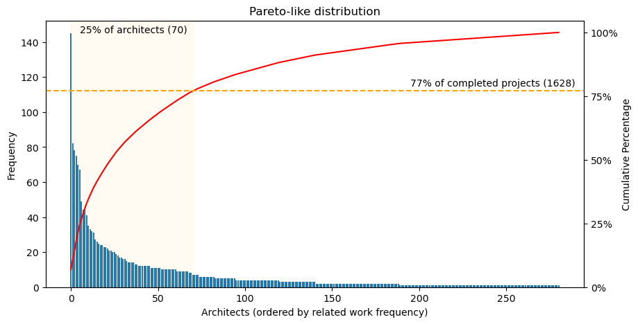
25% of architects are related to 77% of the completed projects.
Registered architects#
Below we identify all registered architects in the DAQA dataset. This information is embedded within the career field of each person record. We visualise a comparison of registration year and degree completion year for each architect. Note that not all architects have corresponding education data.
Show code cell source
registered_architects = []
registered_architects_years = []
for idx,row in daqapersons_1940_80.iterrows():
    try:
        reg_df = pd.json_normalize(ast.literal_eval(row['career'])['registrations'])
        reg_df = reg_df[reg_df['coverage.date.year'].notnull()].sort_values('coverage.date.year')
        if reg_df.shape[0] > 0:
            closest_year = reg_df['coverage.date.year'].values[0]
            registered_architects.append(row[['display_name','ori_id', 'gender']])
            registered_architects_years.append(closest_year)
    except: pass

registered_architects = pd.DataFrame(registered_architects)
registered_architects['reg_year'] = registered_architects_years
registered_architects['gender'] = registered_architects.gender.fillna('Missing')

# fetch education details for registered architects
education_registered = education_training_df_with_dates[education_training_df_with_dates.ori_id.isin(registered_architects.ori_id)]
education_registered = education_registered[education_registered['coverage_range.date_range.date_end.year'] != 'incomplete']
education_registered = education_registered.sort_values('coverage_range.date_range.date_end.year')\
    .drop_duplicates(subset=['ori_id'], keep='first')
registered_architects = pd.merge(registered_architects, education_registered[['ori_id','coverage_range.date_range.date_end.year']], on='ori_id', how='left')

# change column name
registered_architects = registered_architects.rename({'coverage_range.date_range.date_end.year':'completion_year_first_qualification'}, axis=1)

print(f'\nThere are {registered_architects.shape[0]} architects (active in 1940-1980) with registration details in their biographical summary.')
print('-',registered_architects[registered_architects.gender == '"male"'].shape[0], 'of these are male architects.')
print('-',registered_architects[registered_architects.gender == '"female"'].shape[0], 'of these are female architects.')
# print('-',registered_architects[registered_architects.gender == 'Missing'].shape[0], 'of these does not have a recorded gender.\n')
# display(registered_architects.sort_values('reg_year', ascending=True).head())
There are 86 architects (active in 1940-1980) with registration details in their biographical summary.
- 77 of these are male architects.
- 9 of these are female architects.
Show code cell source
# plot a lollipop chart of reg_year and completion_year_first_qualification
registered_architects_with_qual = registered_architects[registered_architects['completion_year_first_qualification'].notnull()]
registered_architects_with_qual['reg_year'] = registered_architects_with_qual['reg_year'].astype(int)
registered_architects_with_qual['completion_year_first_qualification'] = registered_architects_with_qual['completion_year_first_qualification'].astype(int)
registered_architects_with_qual.sort_values('completion_year_first_qualification', ascending=False, inplace=True)
registered_architects_with_qual.reset_index(drop=True, inplace=True)
registered_architects_with_qual['display_name'] = registered_architects_with_qual['display_name'].apply(lambda x: x.replace('"',''))
registered_architects_with_qual['diff'] = registered_architects_with_qual['reg_year'] - registered_architects_with_qual['completion_year_first_qualification']

# The horizontal plot is made using the hline function
# add grid lines for y-axis
plt.grid(axis='y', linestyle='--', alpha=0.4)

plt.scatter(registered_architects_with_qual['completion_year_first_qualification'],
            registered_architects_with_qual.index, color='tab:orange', alpha=0.7, label='value1')
plt.scatter(registered_architects_with_qual['reg_year'],
            registered_architects_with_qual.index, color='tab:green', alpha=0.7 , label='value2')

# add legend under title and make horizontal
plt.legend(loc='upper center', bbox_to_anchor=(0.5, 1.03), ncol=2, frameon=False,
           labels=['Completion year of first qualification', 'Registration year'])

# if architect is female, make line red
plt.hlines(y=registered_architects_with_qual.index,
           xmin=registered_architects_with_qual['completion_year_first_qualification'],
           xmax=registered_architects_with_qual['reg_year'], color='grey',
           alpha=0.4, label=False)

# Add title and axis names
plt.yticks(registered_architects_with_qual.index, registered_architects_with_qual.display_name)

# change colour of yticks based on condition
for idx,row in registered_architects_with_qual.iterrows():
    if "fe" in row['gender']: plt.gca().get_yticklabels()[idx].set_color('tab:red')

# add annoation in bottom left
plt.annotate('*Female architects highlighted in red', (0,0), (15,25),
             xycoords='axes fraction', textcoords='offset points', va='top', color='tab:red')

plt.title("Year comparison of graduation (of first degree) and registration\n\n", loc='left')
plt.xlabel('')
plt.ylabel('')

# make plot longer
plt.gcf().set_size_inches(7, 16)

# Show the graph
plt.show()
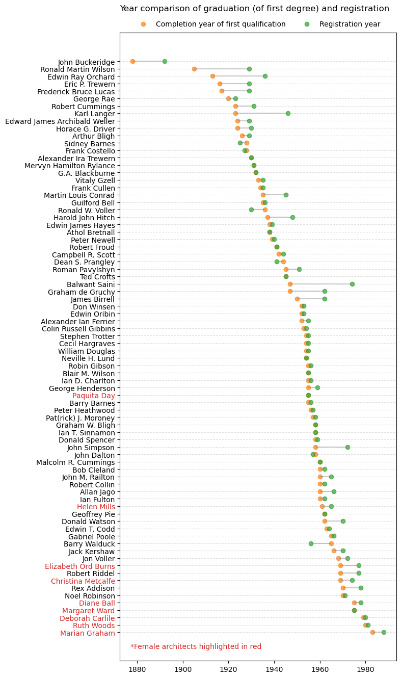
Based on the 78 registered architects with corresponding education data, we find that architects tend to become registered one year after completing their first education qualification.
Typologies#
Below we visualise the frequency of typologies in the DAQA dataset. We continue our analysis by focusing on the period of 1940 to 1980, as well as idenyifing the arcihtects and firms with the most related projects for each typology within this period.
Show code cell source
daqa_work_years = []
daqa_work_ori_ids = []

for idx,row in daqa_work.iterrows():
    try: comp_yr = pd.json_normalize(ast.literal_eval(row['coverage_range'])['date_range'])['date_end.year'].values[0]
    except: comp_yr = None
    daqa_work_years.append(comp_yr)
    daqa_work_ori_ids.append(row['ori_id'])

# create a dummy variable for each typology
typology_dummies_daqa_work = pd.get_dummies(daqa_work['typologies'].\
    fillna('Missing')\
    .str.replace('[^a-zA-Z, ]', '', regex=True)\
    .str.split(', ')\
    .apply(pd.Series).stack())\
    .sum(level=0)

typology_dummies_daqa_work['extracted_compyear'] = daqa_work_years

# create a dataframe with value counts for each typology and year
typology_dummies_counts = typology_dummies_daqa_work.groupby('extracted_compyear')\
    .sum()\
    .reset_index()

typology_dummies_counts['extracted_compyear'] = typology_dummies_counts['extracted_compyear'].astype(int)

# remove erronoous year 1220 and 2029
typology_dummies_counts = typology_dummies_counts.iloc[1:,].head(-1)

# add row for missing years between 1820 and 2022
typology_dummies_counts = typology_dummies_counts\
    .append(pd.DataFrame({'extracted_compyear':list(range(1820,2022))}), ignore_index=True)\
    .fillna(0)\
    .drop_duplicates('extracted_compyear',keep='first')\
    .sort_values('extracted_compyear')

# plot interactve time series for each typology
fig = px.line(typology_dummies_counts, x='extracted_compyear', y=typology_dummies_counts.columns[1:],
title='Number of works by typology and year, 1820-2021',
width=1000, height=500, color_discrete_sequence=px.colors.qualitative.Pastel)

fig.update_yaxes(range=[0, 30])
fig.update_yaxes(title=None)
fig.update_xaxes(title='Year of completion')

# add subtitle
fig.add_annotation(x=0.5, y=1.07, xref='paper', yref='paper',
text='Note: there are some non-disjoint cases in the data.', showarrow=False, font=dict(size=12))

# change legend title from "variable" to "typology"
fig.update_layout(legend_title_text='Typology')

fig.show()
Typologies (1940-1980)#
Show code cell source
# create a dummy variable for each typology
typology_dummies = pd.get_dummies(daqawork_1940_80['typologies'].\
    fillna('Missing')\
    .str.replace('[^a-zA-Z, ]', '', regex=True)\
    .str.split(', ')\
    .apply(pd.Series).stack())\
    .sum(level=0)

# create a dataframe with value counts for each typology and their proportion of the total
typology_dummies_counts = typology_dummies.sum()\
    .reset_index()\
    .rename({'index':'typology',0:'count'}, axis=1)\
    .sort_values('count', ascending=False)\
    .reset_index(drop=True)

# matplotlib plot the freuqencies of typologies with bar labels and switch order of y axis
fig, ax = plt.subplots(figsize=(10,5))
ax.barh(typology_dummies_counts['typology'], typology_dummies_counts['count'], color='steelblue')
ax.set_yticklabels(typology_dummies_counts['typology'], fontsize=12)
ax.set_xlim(0, 300)
ax.set_xlabel('Number of works', fontsize=12)
ax.set_ylabel('')
ax.set_title('Typologies of works, 1940-1980\n\n', fontsize=14)
ax.invert_yaxis()

# add bar labels with proportions in brackets
for p in ax.patches:
    ax.annotate(f'{p.get_width()}', (p.get_width()+3, p.get_y()+0.55), size=12)

ax.text(0.5, 1.05, 'Note: there are some non-disjoint cases in the data.', size=12, ha="center", transform=ax.transAxes)

plt.show()
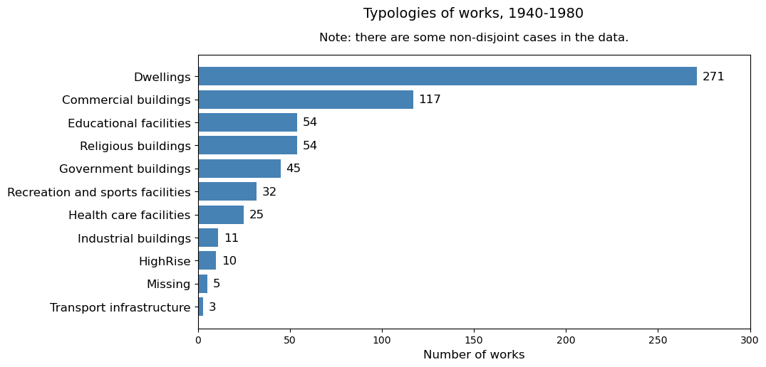
Top 5 architects#
Show code cell source
typology_dummies_daqa_work['ori_id'] = daqa_work_ori_ids
typology_architects = pd.merge(typology_dummies_daqa_work,
                               all_completion_with_name[['subject.label','object.ori_id']],
                               left_on='ori_id', right_on='object.ori_id').drop(['extracted_compyear','ori_id','object.ori_id'], axis=1)

# get the sum of each typology for each firm
typology_architects = typology_architects.groupby('subject.label').sum().reset_index()

for typology in typology_architects.columns[1:]:
    print(f'\n{typology}')

    typology_architects_top5 = typology_architects[['subject.label', typology]]\
        .sort_values(typology, ascending=False)\
        .rename({typology:f'{typology} count'}, axis=1)

    typology_architects_top5 = typology_architects_top5[typology_architects_top5[f'{typology} count'] > 0].head(5)

    display(typology_architects_top5\
    .sort_values(f'{typology} count', ascending=False)\
    .rename({'subject.label':'Architect'}, axis=1)[['Architect', f'{typology} count']])
Commercial buildings
| Architect | Commercial buildings count | |
|---|---|---|
| 60 | Graham W. Bligh | 22 |
| 125 | Robin Gibson | 16 |
| 92 | Karl Langer | 9 |
| 54 | Geoffrey Pie | 4 |
| 132 | Stephen Trotter | 4 |
Dwellings
| Architect | Dwellings count | |
|---|---|---|
| 82 | John Dalton | 62 |
| 92 | Karl Langer | 15 |
| 125 | Robin Gibson | 10 |
| 34 | Donald Spencer | 9 |
| 137 | Vitaly Gzell | 9 |
Educational facilities
| Architect | Educational facilities count | |
|---|---|---|
| 125 | Robin Gibson | 6 |
| 60 | Graham W. Bligh | 6 |
| 118 | Rex Addison | 6 |
| 132 | Stephen Trotter | 5 |
| 90 | Jon Voller | 5 |
Government buildings
| Architect | Government buildings count | |
|---|---|---|
| 92 | Karl Langer | 5 |
| 90 | Jon Voller | 3 |
| 125 | Robin Gibson | 3 |
| 60 | Graham W. Bligh | 3 |
| 127 | Roman Pavylshyn | 3 |
Health care facilities
| Architect | Health care facilities count | |
|---|---|---|
| 131 | Sidney Barnes | 5 |
| 22 | Charles W. T. Fulton | 2 |
| 17 | Bruce Paulsen | 1 |
| 46 | Elmars A. Kraams | 1 |
| 101 | Margaret Ward | 1 |
HighRise
| Architect | HighRise count | |
|---|---|---|
| 68 | Ian D. Charlton | 1 |
| 125 | Robin Gibson | 1 |
| 134 | Ted Crofts | 1 |
| 77 | Jan van den Broek | 1 |
Industrial buildings
| Architect | Industrial buildings count | |
|---|---|---|
| 125 | Robin Gibson | 6 |
| 131 | Sidney Barnes | 1 |
| 137 | Vitaly Gzell | 1 |
| 92 | Karl Langer | 1 |
| 48 | Frank Costello | 1 |
Missing
| Architect | Missing count | |
|---|---|---|
| 104 | Martin Louis Conrad | 1 |
| 115 | Peter Newell | 1 |
| 108 | Neville H. Lund | 1 |
Recreation and sports facilities
| Architect | Recreation and sports facilities count | |
|---|---|---|
| 63 | Guy Crick | 4 |
| 75 | James Birrell | 3 |
| 42 | Edwin Oribin | 3 |
| 118 | Rex Addison | 3 |
| 74 | Jack McElroy | 3 |
Religious buildings
| Architect | Religious buildings count | |
|---|---|---|
| 76 | James Gibson | 14 |
| 92 | Karl Langer | 5 |
| 42 | Edwin Oribin | 4 |
| 1 | Alexander Ian Ferrier | 3 |
| 81 | John Buckeridge | 3 |
Transport infrastructure
| Architect | Transport infrastructure count | |
|---|---|---|
| 10 | Balwant Saini | 1 |
| 92 | Karl Langer | 1 |
| 60 | Graham W. Bligh | 1 |
Top 5 firms#
Show code cell source
# convert projects_1940_80_firms_dict to dataframe
typology_dummies['_id'] = daqawork_1940_80[['_id']]
typology_firms = pd.merge(typology_dummies,
                    pd.DataFrame.from_dict(projects_1940_80_firms_dict, orient='index')\
                        .reset_index()\
                        .rename({'index':'_id', 0:'ori_id'}, axis=1))

# get the sum of each typology for each firm
typology_firms = typology_firms.groupby('ori_id').sum().reset_index()

for typology in typology_dummies_counts['typology'].values:
    print(f'\n{typology}')

    typology_firms_top5 = typology_firms[['ori_id', typology]]\
        .sort_values(typology, ascending=False)\
        .rename({typology:f'{typology} count'}, axis=1)

    typology_firms_top5 = typology_firms_top5[typology_firms_top5[f'{typology} count'] > 0].head(5)

    display(pd.merge(daqa_orgs[['ori_id', 'primary_name']], typology_firms_top5, on='ori_id')\
    .sort_values(f'{typology} count', ascending=False)\
    .rename({'primary_name':'Firm'}, axis=1)[['Firm', f'{typology} count']])
Dwellings
| Firm | Dwellings count | |
|---|---|---|
| 2 | "John Dalton Architect & Associates" | 54 |
| 1 | "Aubrey H. Job & R. P. Froud (Job & Froud)" | 18 |
| 3 | "Hayes & Scott" | 16 |
| 0 | "Karl Langer Architect" | 13 |
| 4 | "John Railton Architect" | 7 |
Commercial buildings
| Firm | Commercial buildings count | |
|---|---|---|
| 2 | "Bligh Jessup Bretnall & Partners" | 18 |
| 1 | "Karl Langer Architect" | 8 |
| 4 | "R F Gibson Architect" | 8 |
| 0 | "Robin Gibson & Partners" | 5 |
| 3 | "Theo Thynne & Associates" | 4 |
Educational facilities
| Firm | Educational facilities count | |
|---|---|---|
| 2 | "Cullen Hargraves Mooney" | 6 |
| 0 | "Fulton Trotter Architects" | 5 |
| 1 | "Robin Gibson & Partners" | 5 |
| 4 | "Bligh Jessup Bretnall & Partners" | 4 |
| 3 | "Goodsir Baker Wilde" | 3 |
Religious buildings
| Firm | Religious buildings count | |
|---|---|---|
| 3 | "THA Cross & D Bain" | 14 |
| 2 | "Karl Langer Architect" | 5 |
| 4 | "S.G. Barnes & Oribin" | 5 |
| 0 | "Ian A Ferrier" | 3 |
| 1 | "W L Douglas & B Barnes" | 3 |
Government buildings
| Firm | Government buildings count | |
|---|---|---|
| 1 | "Karl Langer Architect" | 5 |
| 2 | "Bligh Jessup Bretnall & Partners" | 3 |
| 3 | "Conrad Gargett & Partners (1965-1972)" | 3 |
| 4 | "Commonwealth Department of Works" | 3 |
| 0 | "Robin Gibson & Partners" | 2 |
Recreation and sports facilities
| Firm | Recreation and sports facilities count | |
|---|---|---|
| 1 | "A.H Conrad & T.B.F Gargett" | 3 |
| 4 | "Brisbane City Council, City Design" | 3 |
| 0 | "Karl Langer Architect" | 2 |
| 3 | "S.G. Barnes & Oribin" | 2 |
| 2 | "James Birrell & Partners" | 1 |
Health care facilities
| Firm | Health care facilities count | |
|---|---|---|
| 2 | "S.G. Barnes" | 4 |
| 4 | "J M Collin & C W T Fulton" | 4 |
| 1 | "A.H Conrad & T.B.F Gargett" | 2 |
| 0 | "Donald W Spencer" | 1 |
| 3 | "Theo Thynne & Associates" | 1 |
Industrial buildings
| Firm | Industrial buildings count | |
|---|---|---|
| 0 | "Robin Gibson & Partners" | 3 |
| 4 | "R F Gibson Architect" | 3 |
| 1 | "Karl Langer Architect" | 1 |
| 2 | "S.G. Barnes" | 1 |
| 3 | "Theo Thynne & Associates" | 1 |
HighRise
| Firm | HighRise count | |
|---|---|---|
| 3 | "Prangley & Crofts" | 4 |
| 4 | "Theo Thynne, Denham & Associates" | 2 |
| 0 | "Curro Nutter & Charlton" | 1 |
| 1 | "Robin Gibson & Partners" | 1 |
| 2 | "Peddle Thorp & Walker" | 1 |
Missing
| Firm | Missing count | |
|---|---|---|
| 0 | "Martin L Conrad Architects" | 1 |
| 1 | "Hennessy, Hennessy & Co" | 1 |
| 2 | "Lund, Hutton & Newell" | 1 |
| 3 | "Ford, Hutton & Newell" | 1 |
Transport infrastructure
| Firm | Transport infrastructure count | |
|---|---|---|
| 0 | "Karl Langer Architect" | 1 |
| 1 | "Bligh Jessup Bretnall & Partners" | 1 |
Interviews#
Below we explore the frequency of interviews by interviewers. We focus only on intereviews with architect interviewees.
Show code cell source
# load data
daqa_resources = df_daqa_dict['resource']
daqa_interviews = daqa_resources[daqa_resources['_class_ori'].str.contains('interview', na=False)]

interviewers = []
interview_data = []

for idx,row in daqa_interviews.iterrows():
    try:
        interviewees_isarchitect = pd.json_normalize(json.loads(row['interviewee']))['architect'].values.tolist()
        if True in interviewees_isarchitect:
            interview_data.append(pd.json_normalize(json.loads(row['interviewee'])))
            interviewers.extend(pd.json_normalize(json.loads(row['interviewer']))['label'].values.tolist())
    except: pass


# plot bar plot of interviewers
interviewers = pd.Series(interviewers)
interviewers.value_counts().plot(kind='barh', figsize=(10,5), title='Number of interviews by interviewers (only architect interviewees)')

# inverse y-axis
plt.gca().invert_yaxis()

# add bar labels and propotions
for i, v in enumerate(interviewers.value_counts()):
    plt.text(v + .4, i + .15, str(v), color='black')

plt.xlim(0, 56.5)
plt.text(28, 13.25, 'Note: there are some non-disjoint cases in the data.', size=12, ha="center")
plt.show()
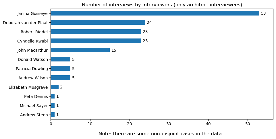
Show code cell source
daqa_persons_interviewed = daqa_persons[daqa_persons["display_name"].apply(lambda x: x.replace('"','')).isin(pd.concat(interview_data)['label'].unique())]

interviewed_orgs = []
for idx,row in daqa_persons_interviewed.iterrows():
    try: interviewed_orgs.append(pd.json_normalize(json.loads(row['related_organizations'])))
    except: pass

interviewed_orgs = pd.concat(interviewed_orgs)
print('Count of interviewed architects by organisation, Top 8:')
interviewed_orgs = interviewed_orgs[interviewed_orgs["predicate.term"] == 'Employment'][["subject.label", "object.label"]].drop_duplicates()
display(interviewed_orgs['object.label'].value_counts().head(8))

avg_no_emnployers = interviewed_orgs.groupby('subject.label').count().reset_index().rename({'object.label':'count'}, axis=1)['count'].median()
Count of interviewed architects by organisation, Top 8:
Conrad Gargett & Partners (1965-1972)               19
Queensland Government Department of Public Works    12
Bligh Jessup Bretnall & Partners                    11
The University of Queensland                         8
Commonwealth Department of Works                     7
A.H Conrad & T.B.F Gargett                           7
Conrad Gargett & Partners (1972-1995)                6
Brisbane City Council                                5
Name: object.label, dtype: int64
On average, interviewed architects have worked for 5 employers.
Socioeconomic factors#
Below we overlay the DAQA dataset (completed projects) with socioeconomic data from the Australian Bureau of Statistics (ABS), Queensland Government Statistician’s Office (QGSO) and Department of Foreign Affairs and Trade (DFAT). Factors include GDP, overseas migration, interstate migration, employment and buildings approved. Most measures are specific to Queensland.
As data is recorded in two forms, by calendar year and financial year, we have developed two applications to explore the data. Applications can be accessed using the following links:
By calendar year: https://daqa-socioecon-cy-dashapp.onrender.com
By financial year: https://daqa-socioeconomic-fy.onrender.com/
The applications consist of the following demographic variables:
ABS data#
Dataset: 3105.0.65.001 Australian Historical Population Statistics, Migration, 2014
Source: https://www.abs.gov.au/AUSSTATS/abs@.nsf/DetailsPage/3105.0.65.0012014
Sheet name: Table 7.2
QLD_Net overseas migration
Net overseas migration (a)(b)(c), Queensland, 1972-2011, FY
(a) From September quarter 1971 to June quarter 2006 inclusive, net overseas migration (NOM) was the difference between permanent and long-term arrivals and permanent and long-term departures. For September quarter 2006 onwards estimates for NOM are the difference between the number of incoming travellers who stay in Australia for 12 months or more and are added to the population (NOM arrivals) and the number of outgoing travellers who leave Australia for 12 months or more and are subtracted from the population (NOM departures). See paragraphs 51 to 54 of the Explanatory Notes.
(b) Estimates for net overseas migration (NOM) contain a break in time series. Estimates for September quarter 2006 onwards use an improved methodology based on the 12/16 rule and are not comparable with NOM estimates prior to this based on the 12/12 rule. See paragraph 51 of the Explanatory Notes.
(c) An adjustment for category jumping (later referred to as migration adjustments) was included for estimates for September quarter 1976 to June quarter 2006, except for September quarter 1997 to June quarter 2001 when it was set to zero. See paragraphs 55 to 57 of the Explanatory Notes.
Sources: ABS data available on request, Population Estimates (for years 1972 - 1981); Australian Demographic Statistics (cat. no. 3101.0) (for years 1982 - 2011)
Sheet name: Table 7.3
QLD_InterstateMigration_Arrivals_To
Interstate migration, arrivals, Queensland, 1972-2010, CY
Sources: ABS data available on request, Population Estimates (for years 1972 - 1981); Australian Demographic Statistics (cat. no. 3101.0) (1982 - 2010)
QLD_InterstateMigration_Departures_from
Interstate migration, departures, Queensland, 1972-2010, CY
Sources: ABS data available on request, Population Estimates (for years 1972 - 1981); Australian Demographic Statistics (cat. no. 3101.0) (1982 - 2010)
QLD_Net interstate migration
Net interstate migration, arrivals, Queensland, 1972-2010, CY
Sources: ABS data available on request, Population Estimates (for years 1972 - 1981); Australian Demographic Statistics (cat. no. 3101.0) (1982 - 2010)
Sheet name: Table 7.5
QLD_Net interstate and overseas migration
Net interstate and overseas migration(a)(b)(c), Queensland, 1860-2010, CY
(a) Until June quarter 1971, net overseas migration (NOM) was the difference between total arrivals and total departures, including short-term movements. From September quarter 1971 to June quarter 2006 inclusive, NOM was the difference between permanent and long-term arrivals and permanent and long-term departures. For September quarter 2006 onwards estimates for NOM are the difference between the number of incoming travellers who stay in Australia for 12 months or more and are added to the population (NOM arrivals) and the number of outgoing travellers who leave Australia for 12 months or more and are subtracted from the population (NOM departures). See paragraphs 51 to 54 of the Explanatory Notes.
(b) Estimates for net overseas migration (NOM) contain a break in time series. Estimates for September quarter 2006 onwards use an improved methodology based on the 12/16 rule and are not comparable with NOM estimates prior to this based on the 12/12 rule. See paragraph 51 of the Explanatory Notes.
(c) An adjustment for category jumping (later referred to as migration adjustments) was included for estimates for September quarter 1976 to June quarter 2006, except for September quarter 1997 to June quarter 2001 when it was set to zero. See paragraphs 55 to 57 of the Explanatory Notes.
Sources: Demography (1910) (for years 1860 - 1901); Australian Demographic Trends, 1997 (cat. no. 3102.0) (for years 1902 - 1980); Australian Demographic Statistics (cat. no. 3101.0) (for years 1981 - 2010)
Sheet name: Table 7.6
QLD_Net interstate and overseas migration rate
Net interstate and overseas migration rate(a)(b)(c)(d), Queensland, 1860-2010, CY
(a) Net movement per 1,000 population. The net interstate and overseas migration rate is the number of net movements in a year per 1,000 mid-year (30 June) estimated resident population. For years prior to 1981, the net interstate and overseas migration rate was based on the mean estimated resident population for the calendar year.
(b) Until June quarter 1971, net overseas migration (NOM) was the difference between total arrivals and total departures, including short-term movements. From September quarter 1971 to June quarter 2006 inclusive, NOM was the difference between permanent and long-term arrivals and permanent and long-term departures. For September quarter 2006 onwards estimates for NOM are the difference between the number of incoming travellers who stay in Australia for 12 months or more and are added to the population (NOM arrivals) and the number of outgoing travellers who leave Australia for 12 months or more and are subtracted from the population (NOM departures). See paragraphs 51 to 54 of the Explanatory Notes.
(c) Estimates for net overseas migration (NOM) contain a break in time series. Estimates for September quarter 2006 onwards use an improved methodology based on the 12/16 rule and are not comparable with NOM estimates prior to this based on the 12/12 rule. See paragraph 51 of the Explanatory Notes.
(d) An adjustment for category jumping (later referred to as migration adjustments) was included for estimates for September quarter 1976 to June quarter 2006, except for September quarter 1997 to June quarter 2001 when it was set to zero. See paragraphs 55 to 57 of the Explanatory Notes.
Sources: Demography (1910) (for years 1860 - 1901); Australian Demographic Trends, 1997 (cat. no. 3102.0) (for years 1902 - 1980); Australian Demographic Statistics (cat. no. 3101.0) (for years 1981 - 2010)
Dataset: 6204055001TS0004 Labour Force Historical Timeseries, Australia - Labour Force Status by State, Queensland
Source: https://www.abs.gov.au/statistics/labour/employment-and-unemployment/labour-force-australia-detailed/latest-release
QLD_Males_Employed_000
Labour Force Status, Employed, Males, Queensland - 1966 – 1977, CY
QLD_Males_Looking for full-time work_000
Labour Force Status, Unemployed - Looking for full-time work, Males, Queensland - 1966 – 1977, CY
QLD_Males_Looking for part-time work_000
Labour Force Status, Unemployed - Looking for part-time work, Males, Queensland - 1966 – 1977, CY
QLD_Males_Total_000
Labour Force Status, Unemployed - Total, Males, Queensland - 1966 – 1977, CY
QLD_Males_Labour force_000
Labour Force Status, Labour force, Males, Queensland - 1966 – 1977, CY
QLD_Males_Not in labour force_000
Labour Force Status, Not in labour force, Males, Queensland - 1966 – 1977, CY
QLD_Males_Civilian pop’n aged 15 years and over_000
Labour Force Status, Civilian population aged 15 years and over, Males, Queensland - 1966 – 1977, CY
QLD_Males_Unemployment rate_%
Labour Force Status, Unemployment Rate, Males, Queensland - 1966 – 1977, CY
QLD_Males_Partic-ipation rate_%
Labour Force Status, Participation Rate, Males, Queensland - 1966 – 1977, CY
QLD_Females_Employed_000
Labour Force Status, Employed, Females, Queensland - 1966 – 1977, CY
QLD_Females_Looking for full-time work_000
Labour Force Status, Unemployed - Looking for full-time work, Females, Queensland - 1966 – 1977, CY
QLD_Females_Looking for part-time work_000
Labour Force Status, Unemployed - Looking for part-time work, Females, Queensland - 1966 – 1977, CY
QLD_Females_Total_000
Labour Force Status, Unemployed - Total, Females, Queensland - 1966 – 1977, CY
QLD_Females_Labour force_000
Labour Force Status, Labour force, Females, Queensland - 1966 – 1977, CY
QLD_Females_Not in labour force_000
Labour Force Status, Not in labour force, Females, Queensland - 1966 – 1977, CY
QLD_Females_Civilian pop’n aged 15 years and over_000
Labour Force Status, Civilian population aged 15 years and over, Females, Queensland - 1966 – 1977, CY
QLD_Females_Unemployment rate_%
Labour Force Status, Unemployment Rate, Females, Queensland - 1966 – 1977, CY
QLD_Females_Partic-ipation rate_%
Labour Force Status, Participation Rate, Females, Queensland - 1966 – 1977, CY
QLD_TotalPersons_Employed_000
Labour Force Status, Employed, Persons, Queensland - 1966 – 1977, CY
QLD_TotalPersons_Looking for full-time work_000
Labour Force Status, Unemployed - Looking for full-time work, Persons, Queensland - 1966 – 1977, CY
QLD_TotalPersons_Looking for part-time work_000
Labour Force Status, Unemployed - Looking for part-time work, Persons, Queensland - 1966 – 1977, CY
QLD_TotalPersons_Total_000
Labour Force Status, Unemployed - Total, Persons, Queensland - 1966 – 1977, CY
QLD_TotalPersons_Labour force_000
Labour Force Status, Labour force, Persons, Queensland - 1966 – 1977, CY
QLD_TotalPersons_Not in labour force_000
Labour Force Status, Not in labour force, Persons, Queensland - 1966 – 1977, CY
QLD_TotalPersons_Civilian pop’n aged 15 years and over_000
Labour Force Status, Civilian population aged 15 years and over, Persons, Queensland - 1966 – 1977, CY
QLD_TotalPersons_Unemployment rate_%
Labour Force Status, Unemployment Rate, Persons, Queensland - 1966 – 1977, CY
QLD_TotalPersons_Partic-ipation rate_%
Labour Force Status, Participation Rate, Persons, Queensland - 1966 – 1977, CY
Dataset: 3105.0.65.001 Australian Historical Population Statistics, Overseas Arrivals and Departures, 2014
Source: https://www.abs.gov.au/AUSSTATS/abs@.nsf/DetailsPage/3105.0.65.0012014
Sheet name: Table 9.4
QLD_Overseas_Arrivals_Males_Total_movement
Overseas arrivals (b)(c)(d), total movement, Males, Queensland (a), 1901-2010 (h), CY
(a) Prior to 1974, data relates to state/territory of disembarkation (for arrivals) or embarkation (for departures). For 1974 and 1975, data relates to state/territory of clearance. From 1976 onwards data relates to state/territory of usual residence.
(b) Includes arrivals of troops for the years 1915 to 1920 and departures of troops for the years 1914 to 1919.
(c) Excludes troop movements for the period September 1939 to June 1947.
(d) Includes U.S. troops visiting Australia on rest and recreation leave during the years 1970 to 1971.
(h) Overseas arrivals and departures data are rounded to whole numbers. As a result, sums of the componenets may not add exactly to totals.
Sources: Demography (1911, 1922, 1933, 1947, 1949, 1960, 1966) (for years 1901 - 1964); Overseas Arrivals and Departures, Australia (1972) (CBCS ref. no. 4.23) (for years 1965 - 1972); Overseas Arrivals and Departures, Australia (1977) (cat. no. 3404.0) (for years 1973 - 1975); ABS data available on request, Overseas Arrivals and Departures collection (for years 1976 - ); Overseas Arrivals and Departures, Australia (cat. no. 3401.0) (for years 1976 - )
QLD_Overseas_Arrivals_Females_Total_movement
Overseas arrivals (b)(c)(d), total movement, Females, Queensland (a), 1901-2010 (h), CY
(a) Prior to 1974, data relates to state/territory of disembarkation (for arrivals) or embarkation (for departures). For 1974 and 1975, data relates to state/territory of clearance. From 1976 onwards data relates to state/territory of usual residence.
(b) Includes arrivals of troops for the years 1915 to 1920 and departures of troops for the years 1914 to 1919.
(c) Excludes troop movements for the period September 1939 to June 1947.
(d) Includes U.S. troops visiting Australia on rest and recreation leave during the years 1970 to 1971.
(h) Overseas arrivals and departures data are rounded to whole numbers. As a result, sums of the componenets may not add exactly to totals.
Sources: Demography (1911, 1922, 1933, 1947, 1949, 1960, 1966) (for years 1901 - 1964); Overseas Arrivals and Departures, Australia (1972) (CBCS ref. no. 4.23) (for years 1965 - 1972); Overseas Arrivals and Departures, Australia (1977) (cat. no. 3404.0) (for years 1973 - 1975); ABS data available on request, Overseas Arrivals and Departures collection (for years 1976 - ); Overseas Arrivals and Departures, Australia (cat. no. 3401.0) (for years 1976 - )
QLD_Overseas_Arrivals_Persons_Total_movement
Overseas arrivals (b)(c)(d), total movement, Persons, Queensland (a), 1901-2010 (h), CY
(a) Prior to 1974, data relates to state/territory of disembarkation (for arrivals) or embarkation (for departures). For 1974 and 1975, data relates to state/territory of clearance. From 1976 onwards data relates to state/territory of usual residence.
(b) Includes arrivals of troops for the years 1915 to 1920 and departures of troops for the years 1914 to 1919.
(c) Excludes troop movements for the period September 1939 to June 1947.
(d) Includes U.S. troops visiting Australia on rest and recreation leave during the years 1970 to 1971.
(h) Overseas arrivals and departures data are rounded to whole numbers. As a result, sums of the componenets may not add exactly to totals.
Sources: Demography (1911, 1922, 1933, 1947, 1949, 1960, 1966) (for years 1901 - 1964); Overseas Arrivals and Departures, Australia (1972) (CBCS ref. no. 4.23) (for years 1965 - 1972); Overseas Arrivals and Departures, Australia (1977) (cat. no. 3404.0) (for years 1973 - 1975); ABS data available on request, Overseas Arrivals and Departures collection (for years 1976 - ); Overseas Arrivals and Departures, Australia (cat. no. 3401.0) (for years 1976 - )
QLD_Overseas_Departures_Males_Total_movement
Overseas departures (b)(c)(d), total movement, Males, Queensland (a), 1901-2010 (h), CY
(a) Prior to 1974, data relates to state/territory of disembarkation (for arrivals) or embarkation (for departures). For 1974 and 1975, data relates to state/territory of clearance. From 1976 onwards data relates to state/territory of usual residence.
(b) Includes arrivals of troops for the years 1915 to 1920 and departures of troops for the years 1914 to 1919.
(c) Excludes troop movements for the period September 1939 to June 1947.
(d) Includes U.S. troops visiting Australia on rest and recreation leave during the years 1970 to 1971.
(h) Overseas arrivals and departures data are rounded to whole numbers. As a result, sums of the componenets may not add exactly to totals.
Sources: Demography (1911, 1922, 1933, 1947, 1949, 1960, 1966) (for years 1901 - 1964); Overseas Arrivals and Departures, Australia (1972) (CBCS ref. no. 4.23) (for years 1965 - 1972); Overseas Arrivals and Departures, Australia (1977) (cat. no. 3404.0) (for years 1973 - 1975); ABS data available on request, Overseas Arrivals and Departures collection (for years 1976 - ); Overseas Arrivals and Departures, Australia (cat. no. 3401.0) (for years 1976 - )
QLD_Overseas_Departures_Females_Total_movement
Overseas departures (b)(c)(d), total movement, Females, Queensland (a), 1901-2010 (h), CY
(a) Prior to 1974, data relates to state/territory of disembarkation (for arrivals) or embarkation (for departures). For 1974 and 1975, data relates to state/territory of clearance. From 1976 onwards data relates to state/territory of usual residence.
(b) Includes arrivals of troops for the years 1915 to 1920 and departures of troops for the years 1914 to 1919.
(c) Excludes troop movements for the period September 1939 to June 1947.
(d) Includes U.S. troops visiting Australia on rest and recreation leave during the years 1970 to 1971.
(h) Overseas arrivals and departures data are rounded to whole numbers. As a result, sums of the componenets may not add exactly to totals.
Sources: Demography (1911, 1922, 1933, 1947, 1949, 1960, 1966) (for years 1901 - 1964); Overseas Arrivals and Departures, Australia (1972) (CBCS ref. no. 4.23) (for years 1965 - 1972); Overseas Arrivals and Departures, Australia (1977) (cat. no. 3404.0) (for years 1973 - 1975); ABS data available on request, Overseas Arrivals and Departures collection (for years 1976 - ); Overseas Arrivals and Departures, Australia (cat. no. 3401.0) (for years 1976 - )
QLD_Overseas_Departures_Persons_Total_movement
Overseas departures (b)(c)(d), total movement, Persons, Queensland (a), 1901-2010 (h), CY
(a) Prior to 1974, data relates to state/territory of disembarkation (for arrivals) or embarkation (for departures). For 1974 and 1975, data relates to state/territory of clearance. From 1976 onwards data relates to state/territory of usual residence.
(b) Includes arrivals of troops for the years 1915 to 1920 and departures of troops for the years 1914 to 1919.
(c) Excludes troop movements for the period September 1939 to June 1947.
(d) Includes U.S. troops visiting Australia on rest and recreation leave during the years 1970 to 1971.
(h) Overseas arrivals and departures data are rounded to whole numbers. As a result, sums of the componenets may not add exactly to totals.
Sources: Demography (1911, 1922, 1933, 1947, 1949, 1960, 1966) (for years 1901 - 1964); Overseas Arrivals and Departures, Australia (1972) (CBCS ref. no. 4.23) (for years 1965 - 1972); Overseas Arrivals and Departures, Australia (1977) (cat. no. 3404.0) (for years 1973 - 1975); ABS data available on request, Overseas Arrivals and Departures collection (for years 1976 - ); Overseas Arrivals and Departures, Australia (cat. no. 3401.0) (for years 1976 - )
QGSO data#
Dataset: cpi-all-groups-brisbane-weighted-average-eight-capital-cities-financial-year-1948-49-2021-22.csv
Source: https://www.qgso.qld.gov.au/statistics/theme/economy/prices-indexes/consumer-price-index-state
Brisbane_Index
Consumer Price Index (a)(b): Brisbane, 1948-49 to 2021-22, FY
(a) 2011-12 = 100
(b) Average of four quarters.
Source: ABS 6401.0, Consumer Price Index, Australia.
Brisbane_YoY_change
Consumer Price Index (a)(b): Brisbane, Annual (%) change, 1949-50 to 2021-22, FY
(a) 2011-12 = 100
(b) Average of four quarters.
Source: ABS 6401.0, Consumer Price Index, Australia.
Weighted average of eight capital cities_Index
Consumer Price Index (a)(b): Weighted average of eight capitals, 1948-49 to 2021-22, FY
(a) 2011-12 = 100
(b) Average of four quarters.
Source: ABS 6401.0, Consumer Price Index, Australia.
Weighted average of eight capital cities_YoY_change
Consumer Price Index (a)(b): Weighted average of eight capitals, Annual (%) change, 1949-50 to 2021-22, FY
(a) 2011-12 = 100
(b) Average of four quarters.
Source: ABS 6401.0, Consumer Price Index, Australia.
Dataset: building-approvals-value-building-approved-type-qld-1970-71-2021-22.csv
QLD_BuildingsApproved_Residential houses_Value
Building approvals: value of building approved (a), Residential houses, Queensland, 1970-71 to 2021-22, FY
(a) Based on original series as at June 2022.
Source: ABS, Building Approvals, Australia.
QLD_BuildingsApproved_Other residential_Value
Building approvals: value of building approved (a), Other residential, Queensland, 1970-71 to 2021-22, FY
(a) Based on original series as at June 2022.
Source: ABS, Building Approvals, Australia.
QLD_BuildingsApproved_Alterations, additions and conversions_Value
Building approvals: value of building approved (a), Alterations, additions and conversions, Queensland, 1973-74 to 2021-22, FY
(a) Based on original series as at June 2022.
Source: ABS, Building Approvals, Australia.
QLD_BuildingsApproved_Total residential_Value
Building approvals: value of building approved (a), Total Residential, Queensland, 1973-74 to 2021-22, FY
(a) Based on original series as at June 2022.
Source: ABS, Building Approvals, Australia.
QLD_BuildingsApproved_Non-residential_Value
Building approvals: value of building approved (a), Non-residential, Queensland, 1970-71 to 2021-22, FY
(a) Based on original series as at June 2022.
Source: ABS, Building Approvals, Australia.
QLD_BuildingsApproved_Total_Value
Building approvals: value of building approved (a), Total, Queensland, 1973-74 to 2021-22, FY
(a) Based on original series as at June 2022.
Source: ABS, Building Approvals, Australia.
DFAT data#
Dataset: australias-trade-and-economic-indicators-historical.xlsx
Sheet name: Population
Aus_Population
Population (1788-2017), Australia, CY (a)(b)
(a) Includes estimates of the Indigenous population from 1961 onwards.
(b) For 2017 only, end September 2017
Aus_Short term overseas visitor arrivals
Short-term overseas visitor arrivals (1925-2017), Australia, CY
Aus_Short term Australian resident departures
Short-term Australian resident departures (1925-2017), Australia, CY
Sheet name: Economic
AUS_GDP_Current
Gross Domestic Product, Australia - current price, 1900-01 - 2016-17, FY (a)(b)
(a) Please note there is a time series break in the current price GDP series between 1958-59 and 1959-60.
(b) Excludes livestock accumulation up to 1948-49.
AUS_GDP_Real_2015-16
Real Gross Domestic Product, Australia - 2015-16 prices, 1900-01 - 2016-17, FY
AUS_GDP_Real_2015-16_Percentage
Real Gross Domestic Product Percentage change (%), 1901-02 - 2016-17, Australia, FY
AUS_Terms of trade Index set to 2015-16
Terms of trade Index (2015-16=100), 1900-01 - 2016-17, Australia, FY
AUS_Terms of trade percentage set to 2015-16
Terms of trade precentage change (%), 1901-02 - 2016-17, Australia, FY
AUS_Unemployment rate
Unemployment rate (%), 1900-01 - 2016-17, Australia, FY
Comparing DAQA and DAAO#
We visualise the number of active males and females over time. We capture this activity by filtering on people that have a career start date and end date. The first plot below shows a count of the cumulative career activity for both DAQA and DAAO. The second visualisation displays the proportion of active males and females over time. The visualisations suggest that the gender disparity is not as pronounced in DAAO as it is in DAQA.
Show code cell source
# persons = fetch_data(acdedata='person')
# daao_daqa = persons[persons.data_source.str.contains('DAQA|DAAO')][['gender', 'data_source', 'birth','death','career']]
# daao_daqa = daao_daqa[daao_daqa['career'].notnull()]

# selected_idx = []
# selected_birth_year = []
# selected_start_year = []
# selected_end_year = []
# selected_death_year = []

# for idx,row in daao_daqa.iterrows():
#     try: selected_birth_year.append(int(pd.json_normalize(json.loads(row['birth']))['coverage.date.year'].values[0]))
#     except: selected_birth_year.append(np.nan)

#     try:
#         career_df = pd.json_normalize(pd.json_normalize(json.loads(row['career']))['career_periods'].values[0])
#         selected_start_year.append(career_df['coverage_range.date_range.date_start.year'].min())
#     except: selected_start_year.append(np.nan)

#     try:
#         career_df = pd.json_normalize(pd.json_normalize(json.loads(row['career']))['career_periods'].values[0])
#         selected_end_year.append(career_df['coverage_range.date_range.date_end.year'].max())
#     except: selected_end_year.append(np.nan)

#     try: selected_death_year.append(int(pd.json_normalize(json.loads(row['death']))['coverage.date.year'].values[0]))
#     except: selected_death_year.append(np.nan)

# # daao_daqa = daao_daqa[daao_daqa.index.isin(selected_idx)].copy()
# daao_daqa['birth_year'] = selected_birth_year
# daao_daqa['career_start'] = selected_start_year
# # return max year of selected_end_year and death_year, there may be nan values
# daao_daqa['career_end'] = selected_end_year
# daao_daqa['death_year'] = selected_start_year

# # manipulate career_start so that each value contains the first 4 digits
# daao_daqa['career_start'] = daao_daqa['career_start'].apply(lambda x: np.nan if isinstance(x,float) else str(x)[:4])
# daao_daqa['career_end'] = daao_daqa['career_end'].apply(lambda x: np.nan if isinstance(x,float) else str(x)[:4])
# daao_daqa['death_year'] = daao_daqa['death_year'].apply(lambda x: np.nan if isinstance(x,float) else str(x)[:4])

# # change all strings that are not numbers to nan
# daao_daqa['career_start'] = daao_daqa['career_start'].apply(lambda x: int(x) if str(x).isdigit() else np.nan)
# daao_daqa['career_end'] = daao_daqa['career_end'].apply(lambda x: int(x) if str(x).isdigit() else np.nan)
# daao_daqa['death_year'] = daao_daqa['death_year'].apply(lambda x: int(x) if str(x).isdigit() else np.nan)

# daao_daqa['gender'] = daao_daqa['gender'].apply(lambda x: str(x.replace('"', '')))
# daao_daqa['data_source'] = daao_daqa['data_source'].apply(lambda x: str(x.replace('"', '')))
# daao_daqa = daao_daqa[daao_daqa['gender']\
#     .str.contains('male|female')][['gender','data_source','birth_year','death_year','career_start','career_end']]

# daao_daqa = daao_daqa[(daao_daqa.death_year.notnull()) | (daao_daqa.career_end.notnull())].copy()
# daao_daqa['career_end'] = daao_daqa['career_end'].fillna(-1)
# daao_daqa['death_year'] = daao_daqa['death_year'].fillna(-1)
# daao_daqa['career_end'] = np.where(daao_daqa['career_end'] > daao_daqa['death_year'], daao_daqa['career_end'], daao_daqa['death_year'])

# daao_daqa = daao_daqa[daao_daqa['career_start'].notnull()][['gender','data_source','career_start','career_end']]
# daao_daqa = daao_daqa[daao_daqa['career_start'] != daao_daqa['career_end']]
# daao_daqa.reset_index(inplace=True, drop=True)

# daao_daqa_wide = pd.DataFrame()

# for i,row in daao_daqa.iterrows():
#     for year in range(int(row['career_start']), int(row['career_end'])+1):
#         daao_daqa_wide.loc[i, year] = 1

# daao_daqa_wide = daao_daqa_wide.fillna(0)
# daao_daqa_wide = pd.merge(daao_daqa, daao_daqa_wide, left_index=True, right_index=True)

# daao_females_wide = daao_daqa_wide[(daao_daqa_wide.gender == 'female') & (daao_daqa_wide.data_source == 'DAAO')].copy()
# daao_males_wide = daao_daqa_wide[(daao_daqa_wide.gender == 'male') & (daao_daqa_wide.data_source == 'DAAO')].copy()
# daqa_females_wide = daao_daqa_wide[(daao_daqa_wide.gender == 'female') & (daao_daqa_wide.data_source == 'DAQA')].copy()
# daqa_males_wide = daao_daqa_wide[(daao_daqa_wide.gender == 'male') & (daao_daqa_wide.data_source == 'DAQA')].copy()

# daao_females_wide = daao_females_wide.drop(['gender','data_source','career_start','career_end'], axis=1)
# daao_males_wide = daao_males_wide.drop(['gender','data_source','career_start','career_end'], axis=1)

# daao_gender_count = pd.merge(daao_males_wide.sum().reset_index().sort_values('index', ascending=True),
#                             daao_females_wide.sum().reset_index().sort_values('index', ascending=True),
#                             on='index', how='outer')

# daao_gender_count.columns = ['year','male','female']
# daao_gender_count['data_source'] = 'DAAO'

# daqa_females_wide = daqa_females_wide.drop(['gender','data_source','career_start','career_end'], axis=1)
# daqa_males_wide = daqa_males_wide.drop(['gender','data_source','career_start','career_end'], axis=1)

# daqa_gender_count = pd.merge(daqa_males_wide.sum().reset_index().sort_values('index', ascending=True),
#                             daqa_females_wide.sum().reset_index().sort_values('index', ascending=True),
#                             on='index', how='outer')

# daqa_gender_count.columns = ['year','male','female']
# daqa_gender_count['data_source'] = 'DAQA'

# daqa_daao_gender_count = pd.concat([daao_gender_count, daqa_gender_count])
# daqa_daao_gender_count.to_csv('data/local/DAQA_gender_comparison.csv', index=False)

daqa_daao_gender_count = fetch_small_data_from_github('DAQA_gender_comparison.csv')

# plot
plt.plot(daqa_daao_gender_count[daqa_daao_gender_count.data_source == 'DAAO']['year'],
daqa_daao_gender_count[daqa_daao_gender_count.data_source == 'DAAO']['male'], label='DAAO Male', color='tab:blue')

plt.plot(daqa_daao_gender_count[daqa_daao_gender_count.data_source == 'DAAO']['year'],
daqa_daao_gender_count[daqa_daao_gender_count.data_source == 'DAAO']['female'],
label='DAAO Female', color='tab:orange')

plt.plot(daqa_daao_gender_count[daqa_daao_gender_count.data_source == 'DAQA']['year'],
daqa_daao_gender_count[daqa_daao_gender_count.data_source == 'DAQA']['male'],
label='DAQA Male', color='tab:blue', alpha=0.75, linestyle='dashed')

plt.plot(daqa_daao_gender_count[daqa_daao_gender_count.data_source == 'DAQA']['year'],
daqa_daao_gender_count[daqa_daao_gender_count.data_source == 'DAQA']['female'],
label='DAQA Female', color='tab:orange', alpha=0.75, linestyle='dashed')

plt.title('Number of active males and females for DAAO and DAQA')
plt.xlabel('Year of career activity')

plt.legend()

# increase the size of the plot
fig = plt.gcf()
fig.set_size_inches(12, 4)

plt.show()
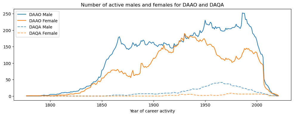
Show code cell source
daqa_daao_gender_count['male_to_female'] = (daqa_daao_gender_count.male/(daqa_daao_gender_count.male + daqa_daao_gender_count.female))

# plot
plt.plot(daqa_daao_gender_count[daqa_daao_gender_count.data_source == 'DAAO']['year'],
daqa_daao_gender_count[daqa_daao_gender_count.data_source == 'DAAO']['male_to_female'], label='DAAO Male-Female Ratio')

plt.plot(daqa_daao_gender_count[daqa_daao_gender_count.data_source == 'DAQA']['year'],
daqa_daao_gender_count[daqa_daao_gender_count.data_source == 'DAQA']['male_to_female'], label='DAQA Male-Female Ratio')

plt.title('Proportion of active males and females for DAAO and DAQA (represented as a ratio), 1800-2000')
plt.ylabel('Male-to-female ratio')
plt.xlabel('Year of career activity')

plt.legend()

# change x-axis limit
plt.xlim(1800, 2025)

# change x-axis tick frequency
plt.xticks(np.arange(1800, 2025, 20))

# add line at 50% mark
plt.axhline(y=0.5, color='grey', linestyle='--', alpha=0.3)

# increase the size of the plot
fig = plt.gcf()
fig.set_size_inches(12, 4)

plt.show()