Tracing the evolution of Melbourne’s music scene

The work presented below form part of ACDE’s presentation at Mapping Culture and History, a workshop held in Novemeber 2022 hosted by Time-Layered Cultural Map of Australia (TLC Map) and ACDE. More details here.

• We focus on the relationship between venues and artists in terms of event frequency and genre evolution.

• Our analysis uses data across three datasets: setlist.fm, Discogs and Spotify.

Import packages and pre-process data

All data used for the following scripts are imported directly from the data/analysis folder located in Github. Although not explicitly described in this notebook, the data collection process is discussed in depth in the video recording below.

After gathering and merging data from the three sources, we pre-process the data to ensure that the data is in a format that is suitable for analysis. A snapshot of two events is provided below to highlight the associated fields for each event. This includes genre and style as defined by the artist’s Discogs profile. To capture temporal changes in musical style, we categorise a musician or band’s genre and style based on the last album released prior to the event.

Furthermore, we supplement each event with relevant Spotify data. This was accomplished by querying the Spotify API for each artist and retrieving acoustic features for each track from the last album released before the event. We then averaged these features across all tracks. For a more in-depth understanding of Spotify’s acoustic features, we direct the reader to their documentation page.

The data in its final form consists of roughly 20,000 events across 300 Melbourne venues.

Show code cell source Hide code cell source

### import modules
# for data/string manipulation
import re
import json
import pandas as pd
import numpy as np
from datetime import datetime
from collections import Counter
import requests, gzip, io, os, json
import ast

# for plotting
import seaborn as sns
import matplotlib as mpl
import matplotlib.pyplot as plt
import plotly.express as px
import sweetviz as sv
px.set_mapbox_access_token("pk.eyJ1Ijoia2FiaXJtYW5hbmRoYXIiLCJhIjoiY2w3ZTMxYWxpMDNtajN3bHZvbHJyYThueiJ9.DpnmOuQdHCWU_crpaEZqAg")
import plotly.graph_objects as go

import plotly.io as pio
import plotly.express as px
import plotly.offline as py

import warnings
warnings.filterwarnings("ignore")

def fetch_small_data_from_github(fname):
    url = f"https://raw.githubusercontent.com/acd-engine/jupyterbook/master/data/analysis/{fname}"
    response = requests.get(url)
    rawdata = response.content.decode('utf-8')
    return io.StringIO(rawdata)

#### Fetch data
#### Setlist fm data
# scraped data collected. Scraping occured on the 7/10/22
mel_df = pd.read_csv(fetch_small_data_from_github('setlistfm_melbourne_events.csv'), index_col=0)

# remove redundant venues
mel_df = mel_df[mel_df.Venue != 'Unknown Venue, Melbourne, Australia']
mel_df = mel_df[mel_df.Venue != "Melbourne Hotel, Perth, Australia"]

# clean venue names
mel_df['Venue'] = mel_df['Venue'].str.replace(r', Melbourne, Australia', '')

# formalise date fields
dates = mel_df['Day'].astype(str)+"-"+mel_df['Month'].astype(str)+"-"+mel_df['Year'].astype(str)
mel_df['Date'] = dates.apply(lambda x: datetime.strptime(x,'%d-%b-%Y'))

# add decade column
mel_df['Decade'] = mel_df.Date.apply(lambda x: x.year // 10 * 10)

# drop any duplicate occurences
mel_df = mel_df.drop_duplicates(subset=['Date','Venue'], keep='first')

# fetch clean venue data
venues_final = pd.read_csv(fetch_small_data_from_github('setlistfm_melbourne_topvenues.csv'), 
                           encoding='latin-1', index_col=0).iloc[:,1:]

new_lats = []
new_longs = []

for idx, ven in venues_final.iterrows():
    if ven.is_problem == 'No geocodes found.':
        new_lats.append(ven.Lat); new_longs.append(ven.Long)
        
    elif ven.is_problem == 'Same match for venue and address.':
        new_lats.append(ven.latitude2); new_longs.append(ven.longitude2)
        
    elif ven.is_problem == 'Address match, but venue no match. Check for accuracy.':
        new_lats.append(ven.latitude); new_longs.append(ven.longitude)
        
    elif ven.is_problem == 'Address match and venue match found but they conflict. Choose the most accurate.':
        new_lats.append(ven.latitude2); new_longs.append(ven.longitude2)
        
    else: pass
    
venues_final['new_lats'] = new_lats
venues_final['new_longs'] = new_longs
venues_final = venues_final[~venues_final.new_lats.isnull()]

# fetch final data
venue_activity_complete = pd.read_csv(fetch_small_data_from_github('setlistfm_mergedwith_discogs_spotify.csv'), index_col=0)
venue_activity_complete = pd.merge(venue_activity_complete, 
                                   venues_final[['Venue','Side of River','new_lats','new_longs']], 
                                   on=['Venue'])

venue_activity_complete.drop(['new_lats_x','new_longs_x'],axis=1, inplace=True)
venue_activity_complete = venue_activity_complete.rename(columns={'new_lats_y': 'new_lats', 'new_longs_y': 'new_longs'})

# DATA ENTRY error
venue_activity_complete.loc[venue_activity_complete.Venue.str.contains('Iceland'),'suburb_nopc'] = 'Ringwood VIC'

venue_activity_complete.tail(2).T

	19858	19859
Month	Nov	Dec
Day	4	29
Year	2019	2019
Artist	KEiiNO	Ali Barter
Tour	Australian Tour 2019	NaN
Venue	The Fyrefly, Melbourne, Australia	The Leadbeater Hotel, Melbourne, Australia
Date	2019-11-04	2019-12-29
Decade	2010	2010
suburb_nopc	NaN	Richmond VIC
Genre	['Folk, World, & Country', 'Pop', 'Electronic']	['Rock', 'Pop']
Style	['Europop', 'Sámi Music', 'Dance-pop']	['Pop Rock', 'Indie Rock', 'Grunge']
quarter	2019 ['Oct', 'Nov', 'Dec']	2019 ['Oct', 'Nov', 'Dec']
new_style	Dance-pop	Indie Rock
album_group	album	album
id	4aYLNUrkHzYLnq9pdFEHyT	12cSgBEuXzWZDVTieZNhIL
name_x	OKTA	Hello, I'm Doing My Best
release_date	2020-05-15	2019-10-18
release_date_precision	day	day
PROMPT	KEiiNO	Ali Barter
danceability	0.6752	0.496545
energy	0.7666	0.674818
key	5.5	6.454545
loudness	-5.9959	-6.519455
mode	0.6	0.909091
speechiness	0.05202	0.048455
acousticness	0.08823	0.084509
instrumentalness	0.000723	0.000155
liveness	0.2115	0.268618
valence	0.5514	0.396818
tempo	116.3908	104.792636
year	2020	2019
Side of River	South	NaN
new_lats	-37.864083	-37.827901
new_longs	144.982999	144.997756

Exploratory Data Analysis

Temporal trends

In this section, we explore the temporal trends in the activity of music venues in Melbourne. We aim to understand how the number of events at these venues has evolved over the years, shedding light on the city’s music scene’s growth and changes.

We begin by analysing the yearly venue activity in Melbourne recorded in setlist.fm which ranges from 1869 to 2022. To achieve this, we create a frequency table of venue occurrences by year and visualise the data using a line plot. The x-axis represents the years, and the y-axis shows the frequency of events (concerts or gigs) held in Melbourne each year. The resulting line plot gives us a glimpse of the overall trend in venue activity over more than a century.

Insight

There is a lack of recorded data prior to the 1970s, with the first significant peak in the number of events occurring in the 1980s. The number of events has been steadily increasing since the mid-90s, with a peak in 2019. The decline in 2020 is attributed to the COVID-19 pandemic.

Show code cell source Hide code cell source

# create a frequency table of venue occurences by year
data_yearly = mel_df[['Year']]\
.value_counts()\
.reset_index()\
.groupby(['Year'])\
.sum()\
.reset_index()

# clean column names
data_yearly.columns = ['Year','Freq']

# visualise data over time
fig = px.line(data_yearly, 
              x="Year", 
              y="Freq",
              title= f'Venue activity in Melbourne, Yearly, 1869-2022')

# set figure size
fig.update_layout(width=800)

fig.show()

Next, we focus on a more recent time frame to highlight the infrequency of event activity in the COVID-19 era. The below plot showcases the frequency of events on a daily basis, allowing us to observe fine-grained patterns relating to factors such as lockdowns.

Show code cell source Hide code cell source

# create a frequency table of venue occurences by individual dates
data_daily = mel_df[['Date']]\
.value_counts()\
.reset_index()\
.groupby(['Date'])\
.sum()\
.reset_index()

# clean column names
data_daily.columns = ['Date','Freq']

# Get weekly count for last two years
daily_placeholder = pd.DataFrame({'Date': pd.date_range('2020-01-01', 
                                                        data_daily.iloc[-1]['Date'])})
data_daily = pd.merge(daily_placeholder, data_daily, on='Date', how='left')
data_daily = data_daily.set_index('Date')
data_daily = data_daily['Freq'].resample('D').sum() #.plot()
data_daily = pd.DataFrame(data_daily).reset_index()

# visualise data over time
fig = px.line(data_daily, 
              x="Date", 
              y="Freq",
              title= f'Venue activity in Melbourne, Daily, 2020-2022 <br><sup>Lockdowns highlighted in red</sup>')

highlighting_params = {'line_width': 0, 'fillcolor': 'red', 
                       'opacity': 0.1, 'annotation_position':"top right",
                       'annotation_textangle': 0}

fig.add_vrect(x0='2020-03-30', x1='2020-05-12', **highlighting_params, annotation_text="1st")
fig.add_vrect(x0='2020-08-08', x1='2020-10-27', **highlighting_params, annotation_text="2nd")
fig.add_vrect(x0='2021-02-12', x1='2021-02-17', **highlighting_params, annotation_text="3rd")
fig.add_vrect(x0='2021-05-27', x1='2021-06-10', **highlighting_params, annotation_text="4th")
fig.add_vrect(x0='2021-07-15', x1='2021-07-27', **highlighting_params, annotation_text="5th")
fig.add_vrect(x0='2021-08-05', x1='2021-10-21', **highlighting_params, annotation_text="6th")

# set figure size
fig.update_layout(width=800)

fig.show()

Due to the lack of data prior to the mid-70s, we decide to focus on setlist.fm data from 1974 to 2019. We also choose to limit the data to 2019 to avoid the impact of the COVID-19 pandemic which distorts the data in terms of genre evolution. Similar to the previous yearly analysis, we create a frequency table of venue occurrences by year and present the data through a line plot.

Show code cell source Hide code cell source

# create a frequency table of venue occurences by year
data_yearly = venue_activity_complete[['Year']]\
.value_counts()\
.reset_index()\
.groupby(['Year'])\
.sum()\
.reset_index()

# clean column names
data_yearly.columns = ['Year','Freq']

# visualise data over time
fig = px.line(data_yearly, 
              x="Year", 
              y="Freq",
              title= f'Venue activity in Melbourne, Yearly, 1974-2019')

# set figure size
fig.update_layout(width=800)

fig.show()

Venue Frequency

Suburb level

Now, let’s focus on analysing event frequency at the suburb level, gaining insights into which suburbs have been most active in hosting music events in Melbourne over the years.

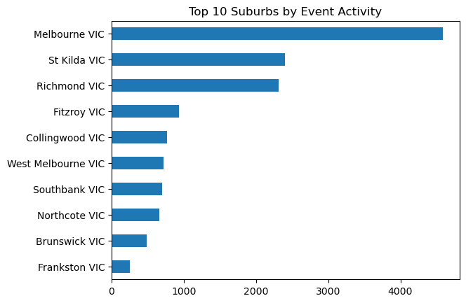
We start by examining the top 10 suburbs with the highest event frequency using a horizontal bar plot.

Insight

Melbourne CBD has the highest number of events, followed by St Kilda, Richmond and Fitzroy. This is not surprising given that these suburbs are known for their vibrant music scene. Out of the top ten, Frankston is the only suburb located outside of the inner city.

Show code cell source Hide code cell source

venue_activity_complete['suburb_nopc'].value_counts().head(10).sort_values().plot(kind="barh")

plt.title('Top 10 Suburbs by Event Activity')

# control figure width
plt.rcParams['figure.figsize'] = [9, 5]

plt.show()

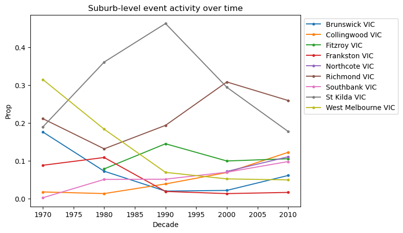
Next, we dive deeper into the event activity proportions over the decades for the top 10 suburbs with the highest music activity. To focus more on local hotspots, we exclude the ‘Melbourne CBD’ entry as a majority of these events are associated with large venues i.e., Rod Laver Arena.

Insight

The line plot belows shows a clear peak in event activity in St Kilda in the 1990s, with a steady decline in the 2000s. Richmond surpasses St Kilda in the 2000s, and remains the most active suburb in the 2010s.

Show code cell source Hide code cell source

dfu = venue_activity_complete[venue_activity_complete.suburb_nopc\
                                .isin(venue_activity_complete['suburb_nopc'].\
                                      value_counts().head(10).index)]

dfu = dfu[dfu.suburb_nopc != 'Melbourne VIC']

# to get the dataframe in the correct shape, unstack the groupby result
dfu = dfu.groupby(['Decade']).suburb_nopc.value_counts(normalize=True).unstack()

# plot
ax = dfu.plot(kind='line', figsize=(7, 5), xlabel='Decade', ylabel='Prop', rot=0, marker='.')
ax.legend(title='', bbox_to_anchor=(1, 1), loc='upper left')

plt.title('Suburb-level event activity over time')

# control figure width
plt.rcParams['figure.figsize'] = [9, 5]

plt.show()

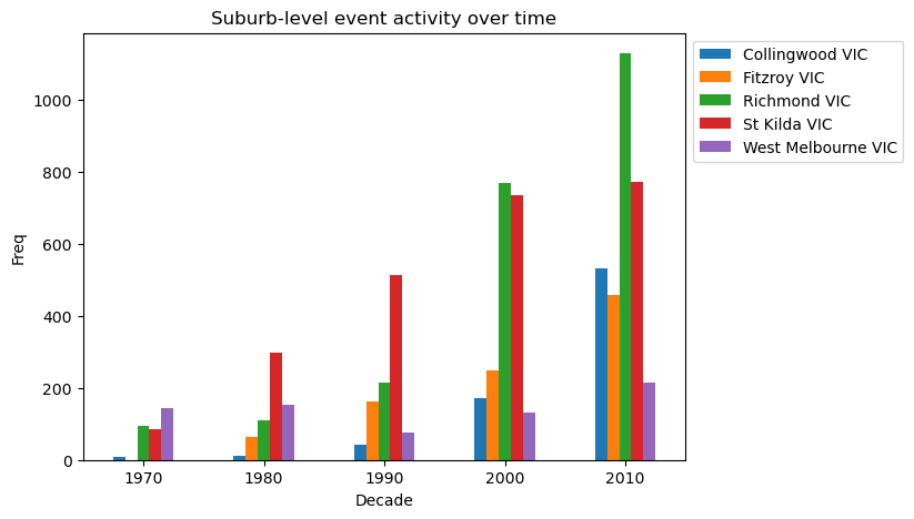
Continuing our analysis, we narrow our focus to the top five suburbs with the highest venue frequency, excluding Melbourne CBD. We group the data by decades and create a clustered bar plot to visualise the actual venue occurrence counts for these suburbs.

Insight

Collingwood and Fitzroy have seen the most significant growth in event activity over the years, with a peak in the 2010s.

Show code cell source Hide code cell source

dfu = venue_activity_complete[venue_activity_complete.suburb_nopc\
                                .isin(venue_activity_complete['suburb_nopc'].\
                                      value_counts().head(6).index)]

dfu = dfu[dfu.suburb_nopc != 'Melbourne VIC']

# to get the dataframe in the correct shape, unstack the groupby result
dfu = dfu.groupby(['Decade']).suburb_nopc.value_counts().unstack()

# plot
ax = dfu.plot(kind='bar', figsize=(7, 5), xlabel='Decade', ylabel='Freq', rot=0)
ax.legend(title='', bbox_to_anchor=(1, 1), loc='upper left')

plt.title('Suburb-level event activity over time')

# control figure width
plt.rcParams['figure.figsize'] = [9, 5]

plt.show()

North or South of the river?

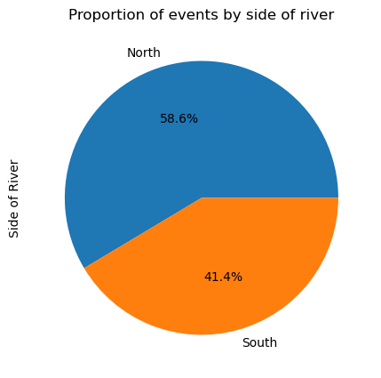
In this section, we explore the distribution of music events in Melbourne based on their location on either the North or South side of the Yarra river.

We begin by analysing the proportion of music events hosted on the North and South sides of the river. To achieve this, we count the occurrences of events in each region and visualize the data using a pie chart.

Show code cell source Hide code cell source

venue_activity_complete['Side of River'].value_counts(normalize=True).plot.pie(autopct='%1.1f%%')

plt.title('Proportion of events by side of river')
plt.show()

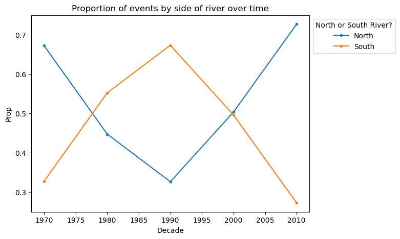
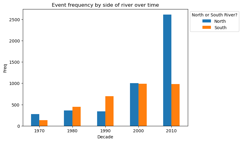
Next, we delve into how the distribution of music events across the North and South sides of the river has evolved over the decades. We also provide the actual frequency of music events on the North and South sides of the river over the decades.

Insight

The St Kilda-Richmond switch in the 2000s is also evident in the North-South analysis.

Show code cell source Hide code cell source

# to get the dataframe in the correct shape, unstack the groupby result
dfu = venue_activity_complete.groupby(['Decade'])['Side of River'].value_counts(normalize=True).unstack()

# plot
ax = dfu.plot(kind='line', figsize=(7, 5), xlabel='Decade', ylabel='Prop', rot=0, marker='.')
ax.legend(title='North or South River?', bbox_to_anchor=(1, 1), loc='upper left')

plt.title('Proportion of events by side of river over time')
plt.show()

dfu = venue_activity_complete.groupby(['Decade'])['Side of River'].value_counts().unstack()

# plot
ax = dfu.plot(kind='bar', figsize=(7, 5), xlabel='Decade', ylabel='Freq', rot=0)
ax.legend(title='North or South River?', bbox_to_anchor=(1, 1), loc='upper left')
plt.title('Event frequency by side of river over time')
plt.show()

Top venues by decade

In this section, we explore the top music venues in Melbourne based on their frequency of hosting events during specific decades.

To begin, we create a frequency table of venue occurrences for each decade, encompassing the entire duration of the dataset. This table gives us an overview of the most active venues throughout different decades.

Show code cell source Hide code cell source

# create a frequency table of venue occurences by decade 
all_events = venue_activity_complete[['Venue','Decade']]\
.value_counts().reset_index()\
.groupby(['Venue','Decade'])\
.sum()\
.reset_index()

# clean column names
all_events.columns = ['Venue','Decade','Freq']

# show first rows
all_events.sort_values('Freq',ascending=False).head(10)

	Venue	Decade	Freq
117	Corner Hotel, Melbourne, Australia	2010	1081
116	Corner Hotel, Melbourne, Australia	2000	744
336	Northcote Social Club, Melbourne, Australia	2010	471
199	Forum Theatre, Melbourne, Australia	2010	445
432	Rod Laver Arena, Melbourne, Australia	2010	409
571	The Hi-Fi, Melbourne, Australia	2000	400
431	Rod Laver Arena, Melbourne, Australia	2000	355
355	Palais Theatre, Melbourne, Australia	2010	349
572	The Hi-Fi, Melbourne, Australia	2010	346
0	170 Russell, Melbourne, Australia	2010	319

Event activity in the 1970s

We then narrow our focus to the 1970s, a transformative decade for music culture. We identify the venues that were most active during this period, and we first visualise their frequency of events over succesive decades using a line plot. This allows us to assess the lifespan of these venues and how their activity has evolved over the years. For example, Festival Hall and Dallas Brook Hall are the only venues that had remained active past the 1980s.

Next, we focus on just the 1970s period and visualise the frequency of events at these venues at a yearly basis to further understand the temporal nuances in event activity. It should be noted that we define the most active venues as those that hosted more than 40 events during the 1970s.

Insight

We can see a clear peak in event activity specifically in 1978 occurring at Tiger Lounge and Bombay Rock. What could be causing this spike? We investigate further.

Show code cell source Hide code cell source

top_venues = all_events[(all_events.Freq >= 1)]['Venue'].unique()
active_in_1970s = all_events[(all_events.Decade == 1970) & (all_events.Freq > 40)]['Venue'].unique()
top_venues_70s = list(set(top_venues) & set(active_in_1970s))

top_in_state = all_events[all_events.Venue.isin(top_venues_70s)]\
.sort_values(['Decade','Venue'])

fig = px.line(top_in_state.sort_values('Decade'), 
              x="Decade", y="Freq", color="Venue",line_group="Venue",
              title= f'<b>Music venues active in 1970s (Melbourne):</b> Decades',
              markers=True)

# set figure size
fig.update_layout(width=800)

fig.show()


all_events_yr = venue_activity_complete[venue_activity_complete.Venue.isin(active_in_1970s)][['Venue','Year']]\
.value_counts().reset_index().groupby(['Venue','Year']).sum().reset_index()
all_events_yr.columns = ['Venue','Year','Freq']
all_events_yr.Year = all_events_yr.Year.astype(int)
all_events_yr = all_events_yr[(all_events_yr.Year > 1965) & (all_events_yr.Year < 1980)]

fig = px.line(all_events_yr.sort_values('Year'), 
              x="Year", y="Freq", color="Venue",line_group="Venue",
              title= f'<b>Music venues most active in 1970s (Melbourne):</b> Years',markers=True)
# set figure size
fig.update_layout(width=800)

fig.show()

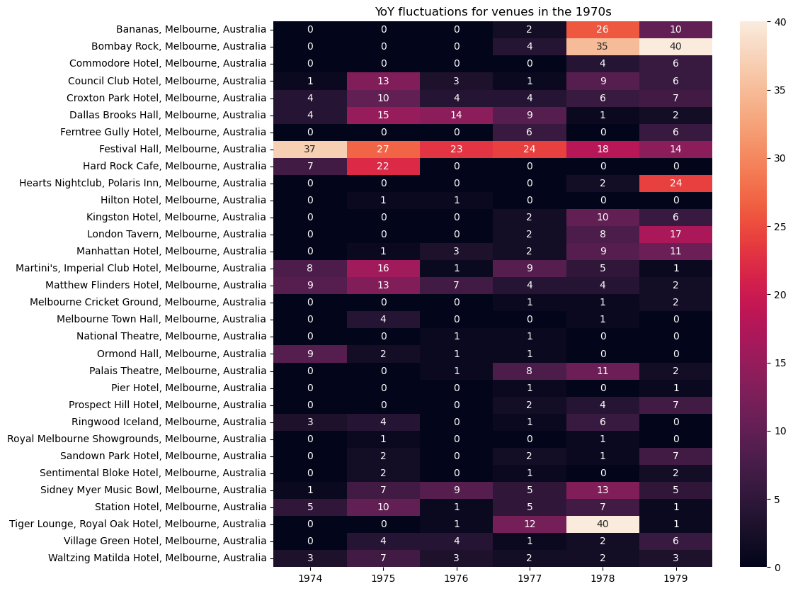
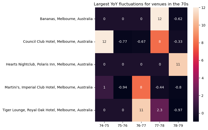
Taking our analysis further, we explore the year-on-year (YoY) fluctuations for venues during the 1970s. We calculate the change in event frequency as a number and as a ratio. This is done for each venue between successive years to determine which venues experienced the most significant shifts, and then visualised through two heatmaps.

Insight

As highlighted in the first heatmap, we can see that Bananas and Hearts Nightclub share a similar peak during the late 1970s. This is better highlighted in the second heatmap which focuses on the top five venues with the highest YoY fluctuations as a ratio. We can see that a shift occurred between 1976 and 1977 for Hearts Nightclub and Tiger Lounge, then in 1978 for Bananas and Council Hotel, and in 1979 for Hearts Nightclub.

Show code cell source Hide code cell source

active_in_1970s = all_events[(all_events.Decade == 1970)]['Venue'].unique()
all_events_yr = venue_activity_complete[venue_activity_complete.Venue.isin(active_in_1970s)][['Venue','Year']]\
.value_counts().reset_index().groupby(['Venue','Year']).sum().reset_index()
all_events_yr.columns = ['Venue','Year','Freq']
all_events_yr.Year = all_events_yr.Year.astype(int)
all_events_yr = all_events_yr[(all_events_yr.Year > 1973) & (all_events_yr.Year < 1980) &
                              (all_events_yr.Venue.isin(all_events_yr[all_events_yr.Freq > 5]['Venue'].unique()))]

piv70s = all_events_yr.pivot(index='Venue', columns='Year', values='Freq').fillna(0)
clipped = piv70s.clip(upper=1).sum(axis=1).reset_index()
piv70s = piv70s[piv70s.index.isin(clipped[clipped[0] > 1].Venue)]

change70s = piv70s.copy()
# change70s['70-71'] = change70s[[1970,1971]].pct_change(axis=1)[1971]
# change70s['71-72'] = change70s[[1971,1972]].pct_change(axis=1)[1972]
# change70s['72-73'] = change70s[[1972,1973]].pct_change(axis=1)[1973]
# change70s['73-74'] = change70s[[1973,1974]].pct_change(axis=1)[1974]
change70s['74-75'] = change70s[[1974,1975]].pct_change(axis=1)[1975]
change70s['75-76'] = change70s[[1975,1976]].pct_change(axis=1)[1976]
change70s['76-77'] = change70s[[1976,1977]].pct_change(axis=1)[1977]
change70s['77-78'] = change70s[[1977,1978]].pct_change(axis=1)[1978]
change70s['78-79'] = change70s[[1978,1979]].pct_change(axis=1)[1979]
change70s = change70s.drop([1974,1975,1976,1977,1978,1979],axis=1).unstack().reset_index()
# change70s = change70s.drop([1970,1971,1972,1973,1974,1975,1976,1977,1978,1979],axis=1).unstack().reset_index()
change70s = change70s[~change70s.isin([np.nan, np.inf, -np.inf]).any(1)]
biggestmovers70s = change70s.sort_values(0, ascending=False).head(5)['Venue'].unique()

fig, ax = plt.subplots(figsize=(10,10))
ax = sns.heatmap(piv70s, annot=True)
ax.set(xlabel="", ylabel="")

plt.title('YoY fluctuations for venues in the 1970s')
plt.show()


forheatmap = change70s[change70s['Venue'].isin(biggestmovers70s)].pivot(index='Venue', columns='Year', values=0).fillna(0)
fig, ax = plt.subplots(figsize=(6,6))
ax = sns.heatmap(forheatmap, annot=True)
ax.set(xlabel="", ylabel="")
plt.title('Largest YoY fluctuations for venues in the 70s')
plt.show()

Similar to the line plot above, we visualise the yearly event frequency for venues, however this time we focus on venues that experienced the sharpest YoY fluctuations. Next, we explore the artists that performed frequently at these venues during the 1970s.

Show code cell source Hide code cell source

all_events_yr = venue_activity_complete[venue_activity_complete.Venue.isin(biggestmovers70s)][['Venue','Year']]\
.value_counts().reset_index().groupby(['Venue','Year']).sum().reset_index()
all_events_yr.columns = ['Venue','Year','Freq']
all_events_yr.Year = all_events_yr.Year.astype(int)
all_events_yr = all_events_yr[(all_events_yr.Year > 1970) & (all_events_yr.Year < 1985)]

fig = px.line(all_events_yr.sort_values('Year'), 
              x="Year", y="Freq", color="Venue",line_group="Venue",
              title= f'<b>Venues, Biggest Movers, 1970s (Melbourne):</b> Year',markers=True)
# set figure size
fig.update_layout(width=800)

fig.show()

Which bands played at Tiger Lounge the most amount of times?

Show code cell source Hide code cell source

venue_activity_complete[venue_activity_complete['Venue'].str.contains('Tiger')].Artist.value_counts().head(3)

The Boys Next Door    39
Midnight Oil           4
Cold Chisel            3
Name: Artist, dtype: int64

Which bands played at Bananas the most amount of times?

Show code cell source Hide code cell source

venue_activity_complete[venue_activity_complete['Venue'].str.contains('Bananas')].Artist.value_counts().head(3)

The Boys Next Door    20
Rose Tattoo           12
Cold Chisel            7
Name: Artist, dtype: int64

Which bands played at Hearts Nightclub (Polaris Inn) the most amount of times?

Show code cell source Hide code cell source

venue_activity_complete[venue_activity_complete['Venue'].str.contains('Polaris Inn')].Artist.value_counts().head(3)

The Boys Next Door    17
Men at Work            7
The Jetsonnes          4
Name: Artist, dtype: int64

Which venue did The Boys Next Door / The Birthday Party play at the most?

Show code cell source Hide code cell source

venue_activity_complete[(venue_activity_complete['Artist'].str.contains('The Boys Next Door')) |
             (venue_activity_complete['Artist'].str.contains('The Birthday Party'))].Venue.value_counts().head(5)

Crystal Ballroom, Melbourne, Australia                 42
Tiger Lounge, Royal Oak Hotel, Melbourne, Australia    39
Bananas, Melbourne, Australia                          20
Hearts Nightclub, Polaris Inn, Melbourne, Australia    19
Bombay Rock, Melbourne, Australia                      17
Name: Venue, dtype: int64

Event activity in the 1980s

We continue our analysis by exploring the most active venues in the 1980s following a similiar methodology as above. It should be noted that we define the most active venues as those that hosted more than 50 events during the 1980s.

Show code cell source Hide code cell source

top_venues = all_events[(all_events.Freq >= 1)]['Venue'].unique()
active_in_1980s = all_events[(all_events.Decade == 1980) & (all_events.Freq > 50)]['Venue'].unique()
top_venues_80s = list(set(top_venues) & set(active_in_1980s))

top_in_state = all_events[all_events.Venue.isin(top_venues_80s)].sort_values(['Decade','Venue'])
top_in_state = top_in_state[top_in_state.Decade > 1969]

fig = px.line(top_in_state.sort_values('Decade'), 
              x="Decade", y="Freq", color="Venue",line_group="Venue",
              title= f'<b>Music venues active in 1980s (Melbourne):</b> Decade',markers=True)

# set figure size
fig.update_layout(width=800)

fig.show()

all_setlists = venue_activity_complete
all_events_yr = all_setlists[all_setlists.Venue.isin(active_in_1980s)][['Venue','Year']]\
.value_counts().reset_index().groupby(['Venue','Year']).sum().reset_index()
all_events_yr.columns = ['Venue','Year','Freq']
all_events_yr.Year = all_events_yr.Year.astype(int)
all_events_yr = all_events_yr[(all_events_yr.Year > 1975) & (all_events_yr.Year < 1990)]

fig = px.line(all_events_yr.sort_values('Year'), 
              x="Year", y="Freq", color="Venue",line_group="Venue",
              title= f'<b>Music venues active in 1980s (Melbourne):</b> Year',markers=True)
# set figure size
fig.update_layout(width=800)

fig.show()

Show code cell source Hide code cell source

active_in_1980s = all_events[(all_events.Decade == 1980)]['Venue'].unique()
all_events_yr = all_setlists[all_setlists.Venue.isin(active_in_1980s)][['Venue','Year']]\
.value_counts().reset_index().groupby(['Venue','Year']).sum().reset_index()
all_events_yr.columns = ['Venue','Year','Freq']
all_events_yr.Year = all_events_yr.Year.astype(int)
all_events_yr = all_events_yr[(all_events_yr.Year > 1979) & (all_events_yr.Year < 1990) &
                              (all_events_yr.Venue.isin(all_events_yr[all_events_yr.Freq > 5]['Venue'].unique()))]

piv80s = all_events_yr.pivot(index='Venue', columns='Year', values='Freq').fillna(0)
clipped = piv80s.clip(upper=1).sum(axis=1).reset_index()
piv80s = piv80s[piv80s.index.isin(clipped[clipped[0] > 1].Venue)]

change80s = piv80s.copy()
change80s['80-81'] = change80s[[1980,1981]].pct_change(axis=1)[1981]
change80s['81-82'] = change80s[[1981,1982]].pct_change(axis=1)[1982]
change80s['82-83'] = change80s[[1982,1983]].pct_change(axis=1)[1983]
change80s['83-84'] = change80s[[1983,1984]].pct_change(axis=1)[1984]
change80s['84-85'] = change80s[[1984,1985]].pct_change(axis=1)[1985]
change80s['85-86'] = change80s[[1985,1986]].pct_change(axis=1)[1986]
change80s['86-87'] = change80s[[1986,1987]].pct_change(axis=1)[1987]
change80s['87-88'] = change80s[[1987,1988]].pct_change(axis=1)[1988]
change80s['88-89'] = change80s[[1988,1989]].pct_change(axis=1)[1989]
change80s = change80s.drop([1980,1981,1982,1983,1984,1985,1986,1987,1988,1989],axis=1).unstack().reset_index() 
change80s = change80s[~change80s.isin([np.nan, np.inf, -np.inf]).any(1)]
biggestmovers80s = change80s.sort_values(0, ascending=False).head(5)['Venue'].unique()

# change last column name
change80s = change80s.rename(columns={0: 'YoY Change'})

print('Largest YoY fluctuations for venues in the 80s')
change80s.sort_values('YoY Change', ascending=False).head(5)

Largest YoY fluctuations for venues in the 80s

	Year	Venue	YoY Change
426	87-88	The Palace Complex, Melbourne, Australia	10.50
405	87-88	Metro Nightclub, Melbourne, Australia	5.00
262	84-85	The Central Club Hotel, Melbourne, Australia	2.25
462	88-89	Old Greek Theatre, Melbourne, Australia	2.00
376	86-87	Village Green Hotel, Melbourne, Australia	2.00

Show code cell source Hide code cell source

all_events_yr = all_setlists[all_setlists.Venue.isin(biggestmovers80s)][['Venue','Year']]\
.value_counts().reset_index().groupby(['Venue','Year']).sum().reset_index()
all_events_yr.columns = ['Venue','Year','Freq']
all_events_yr.Year = all_events_yr.Year.astype(int)
all_events_yr = all_events_yr[(all_events_yr.Year > 1980) & (all_events_yr.Year < 1995)]

fig = px.line(all_events_yr.sort_values('Year'), 
              x="Year", y="Freq", color="Venue",line_group="Venue",
              title= f'<b>Venues, Biggest Movers, 1980s (Melbourne):</b> Year',markers=True)
# set figure size
fig.update_layout(width=800)

fig.show()

Event activity in the 1990s

We continue our analysis by exploring the most active venues in the 1990s. It should be noted that we define the most active venues as those that hosted more than 100 events during the 1990s.

Show code cell source Hide code cell source

top_venues = all_events[(all_events.Freq >= 1)]['Venue'].unique()
active_in_1990s = all_events[(all_events.Decade == 1990) & (all_events.Freq > 100)]['Venue'].unique()
top_venues_90s = list(set(top_venues) & set(active_in_1990s))

top_in_state = all_events[all_events.Venue.isin(top_venues_90s)].sort_values(['Decade','Venue'])
top_in_state = top_in_state[top_in_state.Decade > 1979]

fig = px.line(top_in_state.sort_values('Decade'), 
              x="Decade", y="Freq", color="Venue",line_group="Venue",
              title= f'<b>Music venues active in 1990s (Melbourne):</b> Decade',markers=True)

# set figure size
fig.update_layout(width=800)
fig.show()

all_events_yr = all_setlists[all_setlists.Venue.isin(active_in_1990s)][['Venue','Year']]\
.value_counts().reset_index().groupby(['Venue','Year']).sum().reset_index()
all_events_yr.columns = ['Venue','Year','Freq']
all_events_yr.Year = all_events_yr.Year.astype(int)
all_events_yr = all_events_yr[(all_events_yr.Year > 1985) & (all_events_yr.Year < 2000)]

fig = px.line(all_events_yr.sort_values('Year'), 
              x="Year", y="Freq", color="Venue",line_group="Venue",
              title= f'<b>Music venues active in 1990s (Melbourne):</b> Year',markers=True)

# set figure size
fig.update_layout(width=800)
fig.show()

Show code cell source Hide code cell source

active_in_1990s = all_events[(all_events.Decade == 1990)]['Venue'].unique()
all_events_yr = all_setlists[all_setlists.Venue.isin(active_in_1990s)][['Venue','Year']]\
.value_counts().reset_index().groupby(['Venue','Year']).sum().reset_index()
all_events_yr.columns = ['Venue','Year','Freq']
all_events_yr.Year = all_events_yr.Year.astype(int)
all_events_yr = all_events_yr[(all_events_yr.Year > 1989) & (all_events_yr.Year < 2000) &
                              (all_events_yr.Venue.isin(all_events_yr[all_events_yr.Freq > 5]['Venue'].unique()))]

piv90s = all_events_yr.pivot(index='Venue', columns='Year', values='Freq').fillna(0)
clipped = piv90s.clip(upper=1).sum(axis=1).reset_index()
piv90s = piv90s[piv90s.index.isin(clipped[clipped[0] > 1].Venue)]

change90s = piv90s.copy()
change90s['90-91'] = change90s[[1990,1991]].pct_change(axis=1)[1991]
change90s['91-92'] = change90s[[1991,1992]].pct_change(axis=1)[1992]
change90s['92-93'] = change90s[[1992,1993]].pct_change(axis=1)[1993]
change90s['93-94'] = change90s[[1993,1994]].pct_change(axis=1)[1994]
change90s['94-95'] = change90s[[1994,1995]].pct_change(axis=1)[1995]
change90s['95-96'] = change90s[[1995,1996]].pct_change(axis=1)[1996]
change90s['96-97'] = change90s[[1996,1997]].pct_change(axis=1)[1997]
change90s['97-98'] = change90s[[1997,1998]].pct_change(axis=1)[1998]
change90s['98-99'] = change90s[[1998,1999]].pct_change(axis=1)[1999]
change90s = change90s.drop([1990,1991,1992,1993,1994,1995,1996,1997,1998,1999],axis=1).unstack().reset_index() 
change90s = change90s[~change90s.isin([np.nan, np.inf, -np.inf]).any(1)]
biggestmovers90s = change90s.sort_values(0, ascending=False).head(5)['Venue'].unique()

# change last column name
change90s = change90s.rename(columns={0: 'YoY Change'})

print('Largest YoY fluctuations for venues in the 90s')
change90s.sort_values('YoY Change', ascending=False).head(5)

Largest YoY fluctuations for venues in the 90s

	Year	Venue	YoY Change
360	96-97	Prince Bandroom, Melbourne, Australia	10.00
281	95-96	Corner Hotel, Melbourne, Australia	8.25
428	97-98	The Central Club Hotel, Melbourne, Australia	7.00
170	93-94	Continental Cafe, Melbourne, Australia	6.00
156	92-93	The Esplanade Hotel, Melbourne, Australia	5.00

Show code cell source Hide code cell source

all_events_yr = all_setlists[all_setlists.Venue.isin(biggestmovers90s)][['Venue','Year']]\
.value_counts().reset_index().groupby(['Venue','Year']).sum().reset_index()
all_events_yr.columns = ['Venue','Year','Freq']
all_events_yr.Year = all_events_yr.Year.astype(int)
all_events_yr = all_events_yr[(all_events_yr.Year > 1990) & (all_events_yr.Year < 2000)]

fig = px.line(all_events_yr.sort_values('Year'), 
              x="Year", y="Freq", color="Venue",line_group="Venue",
              title= f'<b>Venues, Biggest Movers, 1990s (Melbourne):</b> Year',markers=True)

# set figure size
fig.update_layout(width=800)
fig.show()

Event activity in the 2000s

We continue our analysis by exploring the most active venues in the 2000s. It should be noted that we define the most active venues as those that hosted more than 150 events during the 2000s.

Show code cell source Hide code cell source

top_venues = all_events[(all_events.Freq >= 1)]['Venue'].unique()
active_in_2000s = all_events[(all_events.Decade == 2000) & (all_events.Freq > 150)]['Venue'].unique()
top_venues_00s = list(set(top_venues) & set(active_in_2000s))

top_in_state = all_events[all_events.Venue.isin(top_venues_00s)].sort_values(['Decade','Venue'])
top_in_state = top_in_state[top_in_state.Decade > 1989]

fig = px.line(top_in_state.sort_values('Decade'), 
              x="Decade", y="Freq", color="Venue",line_group="Venue",
              title= f'<b>Top music venues active in 2000s (Melbourne):</b> Decade',markers=True)

# set figure size
fig.update_layout(width=800)
fig.show()

all_events_yr = all_setlists[all_setlists.Venue.isin(active_in_2000s)][['Venue','Year']]\
.value_counts().reset_index().groupby(['Venue','Year']).sum().reset_index()
all_events_yr.columns = ['Venue','Year','Freq']
all_events_yr.Year = all_events_yr.Year.astype(int)
all_events_yr = all_events_yr[(all_events_yr.Year > 1995) & (all_events_yr.Year < 2010)]

fig = px.line(all_events_yr.sort_values('Year'), 
              x="Year", y="Freq", color="Venue",line_group="Venue",
              title= f'<b>Music venues active in 2000s (Melbourne):</b> Year',markers=True)

# set figure size
fig.update_layout(width=800)
fig.show()

Show code cell source Hide code cell source

active_in_2000s = all_events[(all_events.Decade == 2000)]['Venue'].unique()
all_events_yr = all_setlists[all_setlists.Venue.isin(active_in_2000s)][['Venue','Year']]\
.value_counts().reset_index().groupby(['Venue','Year']).sum().reset_index()
all_events_yr.columns = ['Venue','Year','Freq']
all_events_yr.Year = all_events_yr.Year.astype(int)
all_events_yr = all_events_yr[(all_events_yr.Year > 1999) & (all_events_yr.Year < 2010) &
                              (all_events_yr.Venue.isin(all_events_yr[all_events_yr.Freq > 5]['Venue'].unique()))]

piv00s = all_events_yr.pivot(index='Venue', columns='Year', values='Freq').fillna(0)
clipped = piv00s.clip(upper=1).sum(axis=1).reset_index()
piv00s = piv00s[piv00s.index.isin(clipped[clipped[0] > 1].Venue)]

change00s = piv00s.copy()
change00s['00-01'] = change00s[[2000,2001]].pct_change(axis=1)[2001]
change00s['01-02'] = change00s[[2001,2002]].pct_change(axis=1)[2002]
change00s['02-03'] = change00s[[2002,2003]].pct_change(axis=1)[2003]
change00s['03-04'] = change00s[[2003,2004]].pct_change(axis=1)[2004]
change00s['04-05'] = change00s[[2004,2005]].pct_change(axis=1)[2005]
change00s['05-06'] = change00s[[2005,2006]].pct_change(axis=1)[2006]
change00s['06-07'] = change00s[[2006,2007]].pct_change(axis=1)[2007]
change00s['07-08'] = change00s[[2007,2008]].pct_change(axis=1)[2008]
change00s['08-09'] = change00s[[2008,2009]].pct_change(axis=1)[2009]
change00s = change00s.drop([2000,2001,2002,2003,2004,2005,2006,2007,2008,2009],axis=1).unstack().reset_index() 
change00s = change00s[~change00s.isin([np.nan, np.inf, -np.inf]).any(1)]
biggestmovers00s = change00s.sort_values(0, ascending=False).head(5)['Venue'].unique()

# change last column name
change00s = change00s.rename(columns={0: 'YoY Change'})

print('Largest YoY fluctuations for venues in the 00s')
change00s.sort_values('YoY Change', ascending=False).head(5)

Largest YoY fluctuations for venues in the 00s

	Year	Venue	YoY Change
648	07-08	Palace Theatre, Melbourne, Australia	28.0
777	08-09	Thornbury Theatre, Melbourne, Australia	11.0
652	07-08	Pier Hotel, Melbourne, Australia	7.0
151	01-02	The Empress Hotel, Melbourne, Australia	6.0
732	08-09	Next, Melbourne, Australia	6.0

Show code cell source Hide code cell source

all_events_yr = all_setlists[all_setlists.Venue.isin(biggestmovers00s)][['Venue','Year']]\
.value_counts().reset_index().groupby(['Venue','Year']).sum().reset_index()
all_events_yr.columns = ['Venue','Year','Freq']
all_events_yr.Year = all_events_yr.Year.astype(int)
all_events_yr = all_events_yr[(all_events_yr.Year > 1995) & (all_events_yr.Year < 2010)]

fig = px.line(all_events_yr.sort_values('Year'), 
              x="Year", y="Freq", color="Venue",line_group="Venue",
              title= f'<b>Venues, Biggest Movers, 2000s (Melbourne):</b> Year',markers=True)

# set figure size
fig.update_layout(width=800)
fig.show()

Event activity in the 2010s

We continue our analysis by exploring the most active venues in the 2010s. It should be noted that we define the most active venues as those that hosted more than 250 events during the 2010s.

Show code cell source Hide code cell source

top_venues = all_events[(all_events.Freq >= 1)]['Venue'].unique()
active_in_2010s = all_events[(all_events.Decade == 2010) & (all_events.Freq > 250)]['Venue'].unique()
top_venues_10s = list(set(top_venues) & set(active_in_2010s))

top_in_state = all_events[all_events.Venue.isin(top_venues_00s)].sort_values(['Decade','Venue'])
top_in_state = top_in_state[top_in_state.Decade > 1999]

fig = px.line(top_in_state.sort_values('Decade'), 
              x="Decade", y="Freq", color="Venue",line_group="Venue",
              title= f'<b>Top music venues active in 2010s (Melbourne):</b> Decade',markers=True)

# set figure size
fig.update_layout(width=800)
fig.show()

all_events_yr = all_setlists[all_setlists.Venue.isin(active_in_2000s)][['Venue','Year']]\
.value_counts().reset_index().groupby(['Venue','Year']).sum().reset_index()
all_events_yr.columns = ['Venue','Year','Freq']
all_events_yr.Year = all_events_yr.Year.astype(int)
all_events_yr = all_events_yr[(all_events_yr.Year > 2005) & (all_events_yr.Year < 2015)]

fig = px.line(all_events_yr.sort_values('Year'), 
              x="Year", y="Freq", color="Venue",line_group="Venue",
              title= f'<b>Music venues active in 2010s (Melbourne):</b> Year',markers=True)
# set figure size
fig.update_layout(width=800)
fig.show()

Show code cell source Hide code cell source

active_in_2010s = all_events[(all_events.Decade == 2010)]['Venue'].unique()
all_events_yr = all_setlists[all_setlists.Venue.isin(active_in_2010s)][['Venue','Year']]\
.value_counts().reset_index().groupby(['Venue','Year']).sum().reset_index()
all_events_yr.columns = ['Venue','Year','Freq']
all_events_yr.Year = all_events_yr.Year.astype(int)
all_events_yr = all_events_yr[(all_events_yr.Year > 2009) & (all_events_yr.Year < 2020) &
                              (all_events_yr.Venue.isin(all_events_yr[all_events_yr.Freq > 5]['Venue'].unique()))]

piv10s = all_events_yr.pivot(index='Venue', columns='Year', values='Freq').fillna(0)
clipped = piv10s.clip(upper=1).sum(axis=1).reset_index()
piv10s = piv10s[piv10s.index.isin(clipped[clipped[0] > 1].Venue)]

change10s = piv10s.copy()
change10s['10-11'] = change10s[[2010,2011]].pct_change(axis=1)[2011]
change10s['11-12'] = change10s[[2011,2012]].pct_change(axis=1)[2012]
change10s['12-13'] = change10s[[2012,2013]].pct_change(axis=1)[2013]
change10s['13-14'] = change10s[[2013,2014]].pct_change(axis=1)[2014]
change10s['14-15'] = change10s[[2014,2015]].pct_change(axis=1)[2015]
change10s['15-16'] = change10s[[2015,2016]].pct_change(axis=1)[2016]
change10s['16-17'] = change10s[[2016,2017]].pct_change(axis=1)[2017]
change10s['17-18'] = change10s[[2017,2018]].pct_change(axis=1)[2018]
change10s['18-19'] = change10s[[2018,2019]].pct_change(axis=1)[2019]
change10s = change10s.drop([2010,2011,2012,2013,2014,2015,2016,2017,2018,2019],axis=1).unstack().reset_index() 
change10s = change10s[~change10s.isin([np.nan, np.inf, -np.inf]).any(1)]
biggestmovers10s = change10s.sort_values(0, ascending=False).head(5)['Venue'].unique()

# change last column name
change10s = change10s.rename(columns={0: 'YoY Change'})

print('Largest YoY fluctuations for venues in the 2010s')
change10s.sort_values('YoY Change', ascending=False).head(5)

Largest YoY fluctuations for venues in the 2010s

	Year	Venue	YoY Change
909	18-19	Stay Gold, Melbourne, Australia	27.0
247	12-13	Melbourne Town Hall, Melbourne, Australia	23.0
299	12-13	The Reverence Hotel, Melbourne, Australia	15.0
865	18-19	Gershwin Room, The Esplanade Hotel, Melbourne,...	14.0
344	13-14	Howler, Melbourne, Australia	12.5

Show code cell source Hide code cell source

all_events_yr = all_setlists[all_setlists.Venue.isin(biggestmovers10s)][['Venue','Year']]\
.value_counts().reset_index().groupby(['Venue','Year']).sum().reset_index()
all_events_yr.columns = ['Venue','Year','Freq']
all_events_yr.Year = all_events_yr.Year.astype(int)
all_events_yr = all_events_yr[(all_events_yr.Year > 2005) & (all_events_yr.Year < 2015)]

fig = px.line(all_events_yr.sort_values('Year'), 
              x="Year", y="Freq", color="Venue",line_group="Venue",
              title= f'<b>Venues, Biggest Movers, 2010s (Melbourne):</b> Year',markers=True)

# set figure size
fig.update_layout(width=800)
fig.show()

Genre

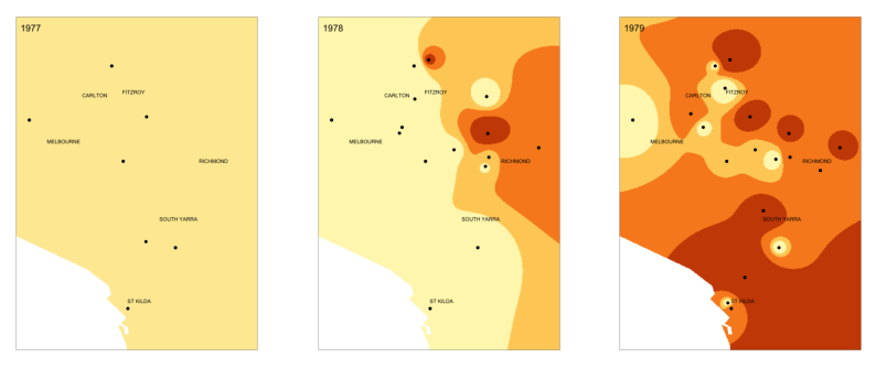
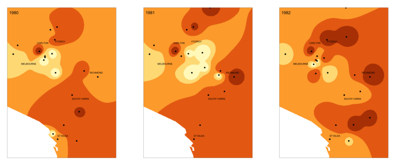
Spatial interpolation

As a starting point, we explore the use of spatial interpolation to model the change in genre of music played in venues over time. As a case study, we explore the movement of alternative music in Melbourne between 1977 and 1982 where darker colours indicate a higher proportion of alternative music played in an area and lighter colours indicate a lower proportion of alternative music played in an area.

Insight

The spatial interpolation maps show that alternative music was mostly concentrated near suburbs such as Richmond and Fitzroy as opposed to Melbourne CBD which hosted more pop music concerts.

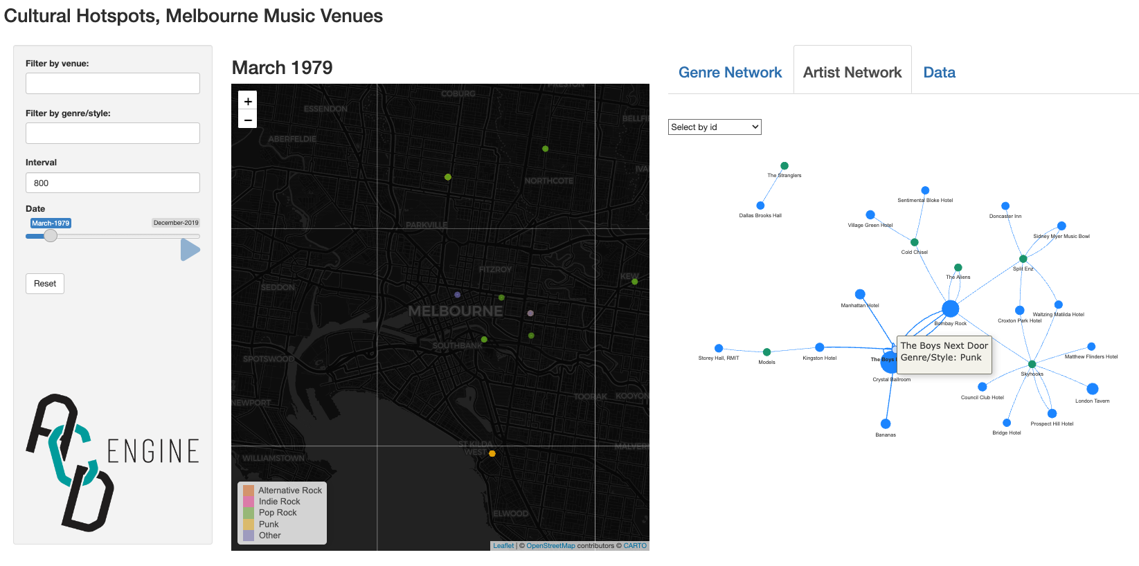
Genre Map and Network analysis

The case study above motivated us to build an interactive mapping application to allow for more functionality in exploring the evolution of genre in Melbourne over time. The application allows for temporal and spatial exploration of genres over time along with the ability to visualise networks across genres, venues and artists. We encourage the reader to explore the application here. A screenshot of the application is provided below.

Spotify acoustic attributes

In this section, we leverage data from Spotify to analyse the density of various acoustic features across venues in Melbourne. Each event contributes to a venue’s acoustic footprint i.e., if a venue hosts a lot of bands that play pop music, then that venue’s acoustic footprint will be high in the danceability attribute. In contrast, a venue that hosts a lot of metal music may be quite low in the danceability attribute.

Below we visualise a series of maps to showcase the spatial distribution of the given acosutic attribute across Melbourne venues. Each map is also animated to allow users to control the temporal dimension of the data.

Show code cell source Hide code cell source

spotify_group_by = venue_activity_complete.groupby(['Venue','Year']).mean().reset_index()

for attr in ['danceability', 'energy', 'loudness', 'speechiness', 'acousticness', 'instrumentalness',
          'liveness', 'valence', 'tempo']:
    fig = px.density_mapbox(venue_activity_complete.sort_values('Date'), lat="new_lats", lon="new_longs",
                            z=attr,title=attr,
                            radius=25,opacity=0.6,hover_name=venue_activity_complete.index,
                            height=800,width=800,color_continuous_scale='inferno', zoom=11,
                           animation_frame = 'Year', center=dict(lat=-37.816244, lon=144.957198))

    fig.update_layout(hovermode='closest', width=800)
    fig.show()